Lab: Representation Showdown

CAP-6640: Computational Understanding of Natural Language
Spencer Lyon

Prerequisites

L03.01: Sparse Representations (BoW, TF-IDF, Scikit-learn)
L03.02: Dense Representations (Word2Vec, GloVe, SpaCy, Gensim)

Outcomes

Apply TF-IDF and word embedding representations to a real text dataset
Compute and interpret document similarity using cosine similarity across representations
Explain how subword tokenization (BPE, WordPiece) handles out-of-vocabulary words
Compare sparse vs. dense representations on similarity and clustering tasks
Use sentence-transformers for document-level embeddings as a preview of modern methods

References

J&M Chapter 5: Embeddings (download)
HF Chapter 6: The Tokenizers Library (link)
spaCy Course Chapter 2: Word Vectors and Semantic Similarity
Sentence-Transformers Documentation

The Arena¶

We’ve spent the last two lectures building up two families of text representation. TF-IDF gives us sparse, high-dimensional vectors where each dimension is a vocabulary word. Word embeddings give us dense, compact vectors where dimensions encode learned semantic features. Both sides have passionate advocates.

But which one actually works better? The honest answer is it depends — and today we’ll see exactly what it depends on. We’ll load a real text dataset, build multiple representations, and pit them head-to-head on two tasks: finding similar documents and organizing documents into clusters. By the end, you’ll have the intuition to choose the right representation for a given problem.

Let’s set up the arena.

import numpy as np
import pandas as pd
import matplotlib.pyplot as plt
from sklearn.datasets import fetch_20newsgroups
from sklearn.feature_extraction.text import TfidfVectorizer
from sklearn.metrics.pairwise import cosine_similarity
from sklearn.manifold import TSNE
import spacy
import warnings

warnings.filterwarnings("ignore", category=FutureWarning)

We’ll use the 20 Newsgroups dataset — a classic benchmark in NLP. It contains roughly 20,000 newsgroup posts across 20 topics. We’ll work with 4 categories that are nicely distinct:

# Load 4 categories from 20 Newsgroups
category_names = [
    "rec.sport.baseball",
    "sci.space",
    "talk.politics.guns",
    "comp.graphics",
]

newsgroups = fetch_20newsgroups(
    subset="train",
    categories=category_names,
    remove=("headers", "footers", "quotes"),  # strip metadata for fair comparison
    random_state=42,
)

# Filter out very short documents (artifacts of header/footer removal)
min_length = 100
mask = [len(text) >= min_length for text in newsgroups.data]
texts = [text for text, keep in zip(newsgroups.data, mask) if keep]
targets = np.array([t for t, keep in zip(newsgroups.target, mask) if keep])
categories = [newsgroups.target_names[t] for t in targets]
short_categories = [c.split(".")[-1] for c in categories]

print(f"Documents after filtering: {len(texts)}")
print(f"\nCategory distribution:")
for cat in category_names:
    short = cat.split(".")[-1]
    count = sum(1 for c in categories if c == cat)
    print(f"  {short:12s}: {count}")

Documents after filtering: 2088

Category distribution:
  baseball    : 505
  space       : 548
  guns        : 509
  graphics    : 526

Let’s peek at a sample document to see what we’re working with:

print(f"Category: {categories[0]}")
print(f"Length: {len(texts[0])} characters")
print(f"\n{texts[0][:500]}...")

Category: talk.politics.guns
Length: 123 characters


What about guns with non-lethal bullets, like rubber or plastic bullets. Would
those work very well in stopping an attack?...

Building the Contenders¶

Contender 1: TF-IDF¶

Our first contender is the veteran — TF-IDF with Scikit-learn. We already know the drill from L03.01: fit a TfidfVectorizer, get a sparse matrix, and we’re ready to compute similarities.

tfidf_vec = TfidfVectorizer(max_features=5000, stop_words="english")
X_tfidf = tfidf_vec.fit_transform(texts)

print(f"TF-IDF matrix shape: {X_tfidf.shape}")
print(f"Non-zero entries: {X_tfidf.nnz:,} out of {X_tfidf.shape[0] * X_tfidf.shape[1]:,}")
print(f"Sparsity: {1 - X_tfidf.nnz / (X_tfidf.shape[0] * X_tfidf.shape[1]):.1%}")

TF-IDF matrix shape: (2088, 5000)
Non-zero entries: 107,558 out of 10,440,000
Sparsity: 99.0%

Each document is now a 5,000-dimensional sparse vector. Over 95% of the entries are zero — most documents use only a small fraction of the vocabulary. But those non-zero entries carry meaningful signal about what each document is about.

Contender 2: Averaged Word Vectors¶

Our second contender uses dense representations. We’ll load SpaCy’s medium model (which includes 300-dimensional word vectors) and represent each document as the average of its token vectors.

Why averaging? It’s the simplest way to get from word-level vectors to a document-level vector: just take the mean across all tokens. SpaCy does this automatically — doc.vector returns the average of all token vectors in the document.

# Load SpaCy with only the components we need (vectors come from the vocab, not a component)
nlp = spacy.load("en_core_web_md", disable=["tagger", "parser", "ner", "attribute_ruler", "lemmatizer"])

# Process all documents — nlp.pipe() is much faster than calling nlp() in a loop
docs = list(nlp.pipe(texts, batch_size=50))
X_spacy = np.array([doc.vector for doc in docs])

print(f"SpaCy matrix shape: {X_spacy.shape}")
print(f"Non-zero entries: {np.count_nonzero(X_spacy):,} out of {X_spacy.size:,}")
print(f"Sparsity: {1 - np.count_nonzero(X_spacy) / X_spacy.size:.1%}")

SpaCy matrix shape: (2088, 300)
Non-zero entries: 626,400 out of 626,400
Sparsity: 0.0%

Notice the contrast: the SpaCy matrix is 300-dimensional (vs. 5,000 for TF-IDF) and almost entirely non-zero. Dense and compact — that’s the whole point.

But averaging has a cost. A document about “space shuttle launches from Cape Canaveral” and a document about “my cat likes to launch itself off the couch into space” would both average out vectors for “space” and “launch” — even though they’re about completely different things. Context and word order are lost. How much does this matter in practice? That’s what we’re here to find out.

Exercise 3.7: Document Length and Averaged Vectors

Averaging word vectors to represent a document is simple but has a subtle implication: document length affects the representation.

Pick a short document and a long document from the dataset. Print their lengths (in tokens, not characters) using the SpaCy Doc objects.
The averaged vector for a 500-word document blends 500 word vectors, while a 20-word document blends only 20. What does this mean for the “specificity” of the resulting vector? Which document’s vector is likely closer to the overall corpus mean?
Can you think of a way to mitigate this effect? (Hint: think about what words contribute the most noise.)

# Starter code
# short_doc = docs[???]  # pick a short one
# long_doc = docs[???]   # pick a long one
# print(f"Short doc: {len(short_doc)} tokens, Long doc: {len(long_doc)} tokens")
#
# # Check distance from the corpus mean
# corpus_mean = X_spacy.mean(axis=0)
# from numpy.linalg import norm
# short_cos = np.dot(short_doc.vector, corpus_mean) / (norm(short_doc.vector) * norm(corpus_mean))
# long_cos = np.dot(long_doc.vector, corpus_mean) / (norm(long_doc.vector) * norm(corpus_mean))

Subword Tokenization: Bridging the Vocabulary Gap¶

Before we bring in our third contender, let’s address a problem we flagged at the end of L03.02: out-of-vocabulary (OOV) words. Static embeddings like Word2Vec and GloVe have a fixed vocabulary. If a word wasn’t in the training data — a misspelling, a technical term, a new slang word — it simply has no vector.

Subword tokenization solves this by breaking words into smaller pieces. Instead of treating “transformerification” as a single unknown token, a subword tokenizer splits it into recognizable parts like “transform”, “er”, “ification”. The model can then compose a meaning from the parts.

The two most important subword algorithms are:

BPE (Byte Pair Encoding): starts with individual characters, iteratively merges the most frequent adjacent pairs. Used by GPT-2, GPT-3/4, LLaMA.
WordPiece: similar to BPE but selects merges that maximize the likelihood of the training data. Used by BERT.

Let’s see them in action:

from transformers import AutoTokenizer

# Load a BPE tokenizer (GPT-2)
bpe_tok = AutoTokenizer.from_pretrained("gpt2")

# Load a WordPiece tokenizer (BERT)
wp_tok = AutoTokenizer.from_pretrained("bert-base-uncased")

# Test on a mix of common and unusual words
test_words = [
    "hello",
    "unbelievable",
    "transformerification",
    "NLP",
    "spaCy",
    "antidisestablishmentarianism",
    "asdfjkl",
]

print(f"{'Word':<30} {'BPE Tokens':<40} {'WordPiece Tokens'}")
print("-" * 100)
for word in test_words:
    bpe_tokens = bpe_tok.tokenize(word)
    wp_tokens = wp_tok.tokenize(word)
    print(f"{word:<30} {str(bpe_tokens):<40} {str(wp_tokens)}")

Word                           BPE Tokens                               WordPiece Tokens
----------------------------------------------------------------------------------------------------
hello                          ['hello']                                ['hello']
unbelievable                   ['un', 'bel', 'iev', 'able']             ['unbelievable']
transformerification           ['trans', 'former', 'ification']         ['transform', '##eri', '##fication']
NLP                            ['N', 'LP']                              ['nl', '##p']
spaCy                          ['sp', 'a', 'Cy']                        ['spa', '##cy']
antidisestablishmentarianism   ['ant', 'idis', 'establishment', 'arian', 'ism'] ['anti', '##dis', '##est', '##ab', '##lish', '##ment', '##arian', '##ism']
asdfjkl                        ['as', 'df', 'j', 'kl']                  ['as', '##df', '##jk', '##l']

Notice the patterns:

Common words (“hello”) stay intact in both tokenizers
Compositional words (“unbelievable”) get split into meaningful parts
Rare/invented words (“transformerification”, “asdfjkl”) get broken into smaller pieces — but they still get some representation, unlike static embeddings which would return nothing
The ## prefix in WordPiece (and Ġ in BPE) marks whether a token is a word start or a continuation

This is why modern transformer models rarely suffer from OOV problems — their tokenizers can handle essentially any string of text. We’ll see these tokenizers again when we work with BERT and GPT in Weeks 6–7.

Exercise 3.8: Subword Tokenization Exploration

Pick a sentence from our 20 Newsgroups dataset and tokenize it with both BPE and WordPiece. How many tokens does each produce? How does this compare to simple whitespace tokenization?
Try tokenizing a sentence with a deliberate misspelling (e.g., “The astronuats launched the spacship”). How do the subword tokenizers handle it compared to looking it up in SpaCy’s vocabulary?
The vocabulary size of GPT-2’s BPE tokenizer is 50,257 tokens, while a word-level tokenizer on the same training data might have 500,000+ entries. Why is the subword vocabulary so much smaller, and what are the trade-offs?

# Starter code
# sample_text = texts[0][:200]
# print(f"Original: {sample_text}")
# print(f"\nWhitespace tokens: {len(sample_text.split())}")
# print(f"BPE tokens: {len(bpe_tok.tokenize(sample_text))}")
# print(f"WordPiece tokens: {len(wp_tok.tokenize(sample_text))}")
#
# misspelled = "The astronuats launched the spacship"
# print(f"\nBPE: {bpe_tok.tokenize(misspelled)}")
# spacy_doc = nlp(misspelled)
# for token in spacy_doc:
#     print(f"  '{token.text}' has_vector={token.has_vector}")

Contender 3: Sentence-Transformers¶

We have one more contender — and it’s a preview of where we’re headed later in the course. Sentence-transformers are transformer-based models specifically trained to produce high-quality sentence and document embeddings. Unlike our SpaCy approach (which just averages word vectors), these models are trained end-to-end to make similar documents produce similar vectors.

We’ll use the all-MiniLM-L6-v2 model, which is small and fast but produces surprisingly good embeddings.

from sentence_transformers import SentenceTransformer

st_model = SentenceTransformer("all-MiniLM-L6-v2")
X_st = st_model.encode(texts, show_progress_bar=True, batch_size=64)

print(f"Sentence-transformer matrix shape: {X_st.shape}")

Warning: You are sending unauthenticated requests to the HF Hub. Please set a HF_TOKEN to enable higher rate limits and faster downloads.

BertModel LOAD REPORT from: sentence-transformers/all-MiniLM-L6-v2
Key                     | Status     |  | 
------------------------+------------+--+-
embeddings.position_ids | UNEXPECTED |  | 

Notes:
- UNEXPECTED	:can be ignored when loading from different task/architecture; not ok if you expect identical arch.

Sentence-transformer matrix shape: (2088, 384)

We now have three contenders ready to compete:

Contender	Dimensions	Type	Approach
TF-IDF	5,000	Sparse	Count word importance
SpaCy Avg. Vectors	300	Dense	Average pre-trained word vectors
Sentence-Transformers	384	Dense	End-to-end trained document encoder

Let the showdown begin.

Round 1: Nearest Neighbors¶

The first test: given a query document, which representation does the best job finding similar documents? We’ll pick a document, find its 5 nearest neighbors under each representation, and compare.

# Pick a space-related document as our query
space_indices = [i for i, c in enumerate(categories) if c == "sci.space"]
query_idx = space_indices[0]

print(f"Query document (category: {short_categories[query_idx]})")
print(f"{texts[query_idx][:300]}...")

Query document (category: space)
Actually, the "ether" stuff sounded a fair bit like a bizzare,
qualitative corruption of general relativity.  nothing to do with
the old-fashioned, ether, though.  maybe somebody could loan him
a GR text at a low level.

didn't get much further than that, tho.... whew.
...

Now let’s find the nearest neighbors under each representation:

# Compute similarities to the query document
tfidf_sims = cosine_similarity(X_tfidf[query_idx], X_tfidf).flatten()
spacy_sims = cosine_similarity(X_spacy[query_idx].reshape(1, -1), X_spacy).flatten()
st_sims = cosine_similarity(X_st[query_idx].reshape(1, -1), X_st).flatten()

# Get top 5 (excluding self)
def top_k_neighbors(sims, k=5):
    indices = np.argsort(sims)[::-1]
    # Skip self (similarity = 1.0)
    return [(idx, sims[idx]) for idx in indices if idx != query_idx][:k]

tfidf_top5 = top_k_neighbors(tfidf_sims)
spacy_top5 = top_k_neighbors(spacy_sims)
st_top5 = top_k_neighbors(st_sims)

# Display side by side
print(f"{'TF-IDF':<35} {'SpaCy Avg Vectors':<35} {'Sentence-Transformers'}")
print("-" * 105)
for i in range(5):
    t_idx, t_sim = tfidf_top5[i]
    s_idx, s_sim = spacy_top5[i]
    st_idx, st_sim = st_top5[i]
    print(
        f"[{short_categories[t_idx]:>10}] {t_sim:.3f}    "
        f"[{short_categories[s_idx]:>10}] {s_sim:.3f}    "
        f"[{short_categories[st_idx]:>10}] {st_sim:.3f}"
    )

TF-IDF                              SpaCy Avg Vectors                   Sentence-Transformers
---------------------------------------------------------------------------------------------------------
[     space] 0.340    [  baseball] 0.988    [     space] 0.588
[      guns] 0.116    [  baseball] 0.987    [     space] 0.377
[  graphics] 0.113    [  baseball] 0.987    [     space] 0.370
[     space] 0.095    [  graphics] 0.987    [     space] 0.365
[  graphics] 0.094    [  baseball] 0.986    [     space] 0.363

Look at the category labels for each column. Are all three representations finding neighbors from the correct category (sci.space)? Or are some representations getting confused, pulling in documents from unrelated topics?

TF-IDF tends to do well here because it matches on specific vocabulary — space-related documents share rare technical terms like “orbit”, “NASA”, “shuttle”. Averaged word vectors can sometimes get confused because averaging washes out specificity. Sentence-transformers typically perform well because they’re trained specifically for semantic similarity.

Exercise 3.9: Your Own Query

Pick a document from a different category (e.g., comp.graphics or talk.politics.guns). Run the same nearest-neighbor analysis for all three representations.
For your query, which representation finds the most on-topic neighbors? Which finds the least? Can you explain why based on what you know about how each representation works?
Find a pair of documents from different categories that have high TF-IDF similarity but low sentence-transformer similarity (or vice versa). What causes the disagreement?

# Starter code
# Pick a document from a different category
# my_query_idx = ???
#
# my_tfidf_sims = cosine_similarity(X_tfidf[my_query_idx], X_tfidf).flatten()
# my_spacy_sims = cosine_similarity(X_spacy[my_query_idx].reshape(1, -1), X_spacy).flatten()
# my_st_sims = cosine_similarity(X_st[my_query_idx].reshape(1, -1), X_st).flatten()
#
# # Find top 5 for each
# for label, sims in [("TF-IDF", my_tfidf_sims), ("SpaCy", my_spacy_sims), ("Sent-Trans", my_st_sims)]:
#     top5 = [(idx, sims[idx]) for idx in np.argsort(sims)[::-1] if idx != my_query_idx][:5]
#     print(f"\n{label}:")
#     for idx, sim in top5:
#         print(f"  [{short_categories[idx]:>10}] {sim:.3f} — {texts[idx][:60]}...")

Round 2: Cluster Visualization¶

Nearest neighbors tell us about individual queries. But we want the big picture: how does each representation organize the entire dataset? Are documents from the same category clustered together? Are the categories well-separated?

We’ll use t-SNE (t-distributed Stochastic Neighbor Embedding) to project each representation down to 2 dimensions for visualization. t-SNE tries to preserve local neighborhood structure — points that are close in the high-dimensional space should stay close in 2D.

# Apply t-SNE to each representation
tsne_params = dict(n_components=2, random_state=42, perplexity=30)

X_tfidf_2d = TSNE(**tsne_params).fit_transform(X_tfidf.toarray())
X_spacy_2d = TSNE(**tsne_params).fit_transform(X_spacy)
X_st_2d = TSNE(**tsne_params).fit_transform(X_st)

# Plot all three side by side
fig, axes = plt.subplots(1, 3, figsize=(18, 5))

unique_cats = sorted(set(short_categories))
colors = plt.cm.tab10(np.linspace(0, 0.4, len(unique_cats)))

for ax, X_2d, title in zip(
    axes,
    [X_tfidf_2d, X_spacy_2d, X_st_2d],
    ["TF-IDF", "SpaCy Avg. Vectors", "Sentence-Transformers"],
):
    for color, cat in zip(colors, unique_cats):
        mask = np.array([c == cat for c in short_categories])
        ax.scatter(X_2d[mask, 0], X_2d[mask, 1], c=[color], label=cat, alpha=0.6, s=20)
    ax.set_title(title, fontsize=14)
    ax.set_xticks([])
    ax.set_yticks([])
    ax.legend(fontsize=8, loc="best")

plt.suptitle("Document Representations Projected to 2D with t-SNE", fontsize=14, y=1.02)
plt.tight_layout()
plt.show()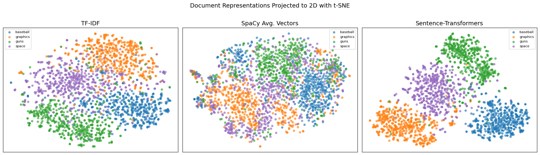

This visualization is revealing. Compare the three plots:

TF-IDF typically produces reasonably distinct clusters because topics use different vocabularies. Space documents talk about “orbit” and “NASA”; baseball documents talk about “pitcher” and “batting”. The lexical signal is strong.
SpaCy averaged vectors may show more overlap between clusters. Averaging many word vectors together tends to push all documents toward a “generic text” center, reducing the distinctiveness of each topic.
Sentence-transformers often produce the tightest, most separated clusters because the model was trained specifically to place semantically similar texts close together.

The pattern isn’t always this clean — t-SNE is stochastic and sensitive to its parameters. But the general trend is consistent: representations that encode more semantic information produce better-organized embedding spaces.

The Verdict¶

We’ve now seen three representations compete on real data. Let’s summarize what we’ve learned about when each shines:

	TF-IDF	SpaCy Avg. Vectors	Sentence-Transformers
Strengths	Fast, interpretable, good lexical matching	Captures synonymy, compact	Best semantic similarity, handles paraphrases
Weaknesses	No synonymy, high-dimensional	Averaging loses specificity	Slower, requires GPU for large-scale use
Best for	Keyword search, topic classification	Quick semantic baseline	Semantic search, clustering, retrieval
Setup cost	Minimal (sklearn only)	Medium (SpaCy model download)	Higher (transformer model download)

The key insight is that there’s no universally best representation. TF-IDF is still a strong baseline for tasks where lexical overlap matters — and it’s orders of magnitude faster to compute than transformer-based embeddings. But when you need to understand that “the spacecraft launched successfully” and “the rocket took off without issues” are about the same thing, you need dense representations.

And within dense representations, the gap between averaged word vectors and purpose-built sentence encoders is significant. Averaging is a crude operation that discards word order and dilutes meaning. Sentence-transformers are trained end-to-end to produce high-quality document embeddings — and it shows.

Exercise 3.10: The Showdown Report

Write a short comparative analysis (1–2 paragraphs for each question) based on your observations from this lab:

When is TF-IDF sufficient? Describe a scenario where TF-IDF would be your first choice over dense embeddings. Consider compute cost, interpretability, and the nature of the task.
When do embeddings clearly win? Give a concrete example (from this lab or hypothetical) where TF-IDF fails but dense representations succeed. What property of embeddings makes the difference?
Averaged word vectors vs. sentence-transformers: We saw that simply averaging word vectors is a step up from TF-IDF but falls short of sentence-transformers. Why? What does the transformer model capture that averaging misses?
The practical trade-off: You’re building an NLP system that needs to process 1 million documents. You have a modest budget and a tight deadline. Which representation would you start with, and under what conditions would you invest in upgrading to a more sophisticated one?

Wrap-Up¶

Key Takeaways¶

Key Takeaways

TF-IDF is a strong baseline — fast, interpretable, and effective when topics have distinct vocabularies
Averaged word vectors capture synonymy but lose specificity as document length increases — averaging is a blunt instrument
Sentence-transformers produce the best document embeddings among the methods we tested, because they’re trained end-to-end for semantic similarity
Subword tokenization (BPE, WordPiece) eliminates the OOV problem by decomposing any word into known subword pieces — the foundation of modern transformer tokenizers
No representation is universally best — the right choice depends on the task, the data, computational budget, and whether you need lexical matching or semantic understanding
Visualization with t-SNE reveals how well a representation organizes documents — tight, well-separated clusters indicate a representation that captures category structure
Practical NLP is about trade-offs — start simple (TF-IDF), measure, and only add complexity when it demonstrably helps

What’s Next¶

In Week 4, we’ll put these representations to work on a core NLP task: text classification. We’ll train classifiers — Naive Bayes, SVM, Logistic Regression — on top of the feature representations we’ve built here. You’ll see that the choice of representation has a direct impact on classification accuracy. We’ll also explore sequence labeling tasks like named entity recognition, where the order of words that our bag-of-words models discard becomes essential.