Text Classification: From Documents to Decisions

CAP-6640: Computational Understanding of Natural Language
Spencer Lyon

Prerequisites

L03.01–03: Text representations (BoW, TF-IDF, word embeddings, cosine similarity)
Week 2: Tokenization, text normalization, SpaCy pipelines
Basic probability (conditional probability, Bayes’ theorem)

Outcomes

Formulate text classification problems, distinguishing binary, multi-class, and multi-label settings
Explain the intuition behind Naive Bayes and Logistic Regression for text, including key formulas
Engineer text features using n-grams and TF-IDF with Scikit-learn’s pipeline API
Build and compare sentiment classifiers using both sparse and dense representations
Evaluate classifiers using accuracy, precision, recall, F1 score, and confusion matrices

References

J&M Chapter 4: Logistic Regression and Text Classification (download)
Scikit-learn: Classification of Text Documents
SpaCy TextCategorizer Documentation

From Vectors to Decisions¶

Last week we learned how to turn text into numbers — sparse vectors with TF-IDF, dense vectors with word embeddings. That’s a powerful foundation, but it raises an obvious question: now that we have these vectors, what do we do with them?

Consider these scenarios:

An email arrives. Is it spam or not spam?
A customer writes a product review. Is the sentiment positive, negative, or neutral?
A news article is published. Is it about politics, sports, technology, or business?

Each of these is a text classification problem — we take a document as input and assign it to one of a predefined set of categories. It’s one of the most common and practically useful tasks in NLP, and it’s where machine learning meets language processing head-on.

In this lecture, we’ll build working classifiers from scratch. By the end, you’ll have a sentiment analysis system trained on real movie reviews, and you’ll understand the algorithms and evaluation metrics that make it work.

The Classification Setup¶

Let’s be precise about what we’re solving. In supervised text classification:

We have a set of documents $x_1, x_2, \ldots, x_n$ (emails, reviews, articles)
Each document has a label $y_i$ from a fixed set of classes $C = \{c_1, c_2, \ldots, c_k\}$
We have a training set of labeled examples
Our goal: learn a function $f(x) \rightarrow c$ that predicts the class of new, unseen documents

The pipeline looks like this:

\text{raw text} \xrightarrow{\text{preprocessing}} \text{tokens} \xrightarrow{\text{representation}} \text{feature vector } \mathbf{x} \xrightarrow{\text{classifier}} \text{class } c

(1)

We already know how to do the first two steps from Weeks 2 and 3. Today we focus on that last arrow — the classifier.

Flavors of Classification¶

Not all classification problems are created equal:

Binary classification: two classes (spam/not-spam, positive/negative). The simplest and most common case.
Multi-class classification: more than two mutually exclusive classes (politics/sports/tech/business). Each document belongs to exactly one class.
Multi-label classification: documents can belong to multiple classes simultaneously. A news article might be tagged as both “politics” and “economics.”

We’ll focus on binary and multi-class today. Multi-label adds complexity in both training and evaluation — it’s more of an engineering challenge than a conceptual one.

Naive Bayes: The Probabilistic Baseline¶

Let’s start with the simplest effective classifier for text: Naive Bayes. It’s fast, surprisingly accurate, and deeply intuitive once you see the logic.

The Core Question¶

Given a document $d$ , which class $c$ is most likely? We want:

\hat{c} = \arg\max_{c \in C} P(c \mid d)

(2)

Direct estimation of $P(c \mid d)$ is hard — we’d need to see many examples of each exact document. But Bayes’ theorem lets us flip the problem:

P(c \mid d) = \frac{P(d \mid c) \cdot P(c)}{P(d)}

(3)

Since $P(d)$ is the same for all classes, we can drop it and just compare:

\hat{c} = \arg\max_{c \in C} \; P(d \mid c) \cdot P(c)

(4)

$P(c)$ is the prior — how common is each class in our training data? If 80% of emails are not spam, the prior for “not-spam” is 0.8.

$P(d \mid c)$ is the likelihood — how probable is this document given the class? This is still hard to estimate directly — every document is a unique sequence of words.

The “Naive” Assumption¶

Here’s the trick that makes everything tractable: assume that each word in the document is conditionally independent given the class. Under this assumption:

P(d \mid c) = P(w_1, w_2, \ldots, w_n \mid c) \approx \prod_{i=1}^{n} P(w_i \mid c)

(5)

This is a terrible assumption linguistically — the probability of seeing “York” absolutely depends on whether “New” just appeared. But it works remarkably well in practice because the classifier doesn’t need to model language perfectly. It just needs to get the relative ranking of classes right.

The full Naive Bayes decision rule becomes:

\hat{c} = \arg\max_{c \in C} \; P(c) \prod_{i=1}^{n} P(w_i \mid c)

(6)

Estimating the Parameters¶

The parameters are easy to estimate from a training set:

P(c) = \frac{\text{number of documents in class } c}{\text{total documents}}

(7)

P(w \mid c) = \frac{\text{count of } w \text{ in documents of class } c}{\text{total words in documents of class } c}

(8)

There’s one problem: if a word never appears in a class’s training documents, $P(w \mid c) = 0$ , which zeros out the entire product. The fix is Laplace (add-one) smoothing:

P(w \mid c) = \frac{\text{count}(w, c) + 1}{\text{total words in } c + |V|}

(9)

where $|V|$ is the vocabulary size. This ensures no probability is ever exactly zero.

Naive Bayes in Practice¶

Let’s see it in action on a toy example before scaling up:

from sklearn.naive_bayes import MultinomialNB
from sklearn.feature_extraction.text import CountVectorizer

# Tiny training set
train_docs = [
    "great movie loved it",
    "wonderful film fantastic acting",
    "terrible movie waste of time",
    "awful boring hated it",
    "amazing performance brilliant",
    "bad film poor acting dull",
]
train_labels = ["pos", "pos", "neg", "neg", "pos", "neg"]

# Convert text to BoW features
vectorizer = CountVectorizer()
X_train = vectorizer.fit_transform(train_docs)

# Train Naive Bayes
nb_clf = MultinomialNB()
nb_clf.fit(X_train, train_labels)

# Predict on new documents
test_docs = [
    "great acting wonderful movie",
    "terrible waste boring",
    "the film was okay",
]
X_test = vectorizer.transform(test_docs)
predictions = nb_clf.predict(X_test)

for doc, pred in zip(test_docs, predictions):
    print(f"  '{doc}' → {pred}")

  'great acting wonderful movie' → pos
  'terrible waste boring' → neg
  'the film was okay' → pos

Even with just 6 training examples, the model picks up the signal. Words like “great”, “wonderful”, and “amazing” push toward positive; words like “terrible”, “boring”, and “awful” push toward negative. The third document — “the film was okay” — is interesting: “okay” never appeared in training, but the model still makes a prediction based on the words it does recognize.

Exercise 4.1: Naive Bayes by Hand

Consider a training set with two classes, “sports” and “tech”:

Sports: “the team won the game”, “great play by the team”
Tech: “the new software update”, “great features in the app”

The word “great” appears in both classes. A new document arrives: “great game update”.

Compute $P(\text{sports})$ and $P(\text{tech})$ — the class priors.
For each class, compute $P(\text{great} \mid c)$ , $P(\text{game} \mid c)$ , and $P(\text{update} \mid c)$ using add-one smoothing with $|V|$ = number of unique words across both classes.
Which class does Naive Bayes assign? Show your work.
What happens if you remove the word “great” from the document? Does the prediction change?

Logistic Regression: Learning Feature Weights¶

Naive Bayes is generative — it models how documents are “generated” by each class. Logistic Regression takes a different approach: it directly learns a mapping from features to class probabilities.

The Intuition¶

Think of it this way: each feature (word) gets a weight that reflects how much evidence it provides for each class. The word “excellent” might get a large positive weight for the positive sentiment class, while “terrible” gets a large negative weight. Classification is just a weighted vote:

z = w_1 x_1 + w_2 x_2 + \cdots + w_n x_n + b = \mathbf{w} \cdot \mathbf{x} + b

(10)

where $\mathbf{x}$ is our feature vector (TF-IDF, BoW, etc.) and $\mathbf{w}$ is a vector of learned weights. But $z$ can be any real number — we need a probability. The sigmoid function squashes it into $[0, 1]$ :

P(y = 1 \mid \mathbf{x}) = \sigma(z) = \frac{1}{1 + e^{-z}}

(11)

The sigmoid has a satisfying shape: large positive $z$ gives probability near 1, large negative $z$ gives probability near 0, and $z = 0$ gives exactly 0.5 — the decision boundary.

Why Not Just Naive Bayes?¶

Both algorithms work well for text, but they have different strengths:

Aspect	Naive Bayes	Logistic Regression
Training	Count and divide — very fast	Optimization (gradient descent) — slower
Assumption	Feature independence	No independence assumption
Small data	Often better	Can overfit
Large data	Good	Often better
Interpretability	Class-conditional probabilities	Feature weights

In practice, Logistic Regression tends to win on larger datasets because it can learn to ignore correlated features, while Naive Bayes counts them all equally. For text, where many words are correlated (“New” and “York”, “ice” and “cream”), this matters.

Logistic Regression in Scikit-learn¶

from sklearn.linear_model import LogisticRegression
from sklearn.feature_extraction.text import TfidfVectorizer

# Same training data, now with TF-IDF features
tfidf_vec = TfidfVectorizer()
X_train_tfidf = tfidf_vec.fit_transform(train_docs)

# Train Logistic Regression
lr_clf = LogisticRegression()
lr_clf.fit(X_train_tfidf, train_labels)

# Predict
X_test_tfidf = tfidf_vec.transform(test_docs)
predictions = lr_clf.predict(X_test_tfidf)

for doc, pred in zip(test_docs, predictions):
    print(f"  '{doc}' → {pred}")

  'great acting wonderful movie' → pos
  'terrible waste boring' → neg
  'the film was okay' → pos

One powerful feature of Logistic Regression is that we can inspect the learned weights to understand why the model makes its decisions:

import pandas as pd
import numpy as np

# Get feature names and weights
features = tfidf_vec.get_feature_names_out()
weights = lr_clf.coef_[0]

# Show top positive and negative weights
weight_df = pd.DataFrame({"feature": features, "weight": weights})
weight_df = weight_df.sort_values("weight", ascending=False)

print("Top 5 features for POSITIVE:")
print(weight_df.head(5).to_string(index=False))
print("\nTop 5 features for NEGATIVE:")
print(weight_df.tail(5).to_string(index=False))

Top 5 features for POSITIVE:
  feature   weight
fantastic 0.235561
wonderful 0.235561
    loved 0.235458
    great 0.235458
  amazing 0.231583

Top 5 features for NEGATIVE:
feature    weight
   dull -0.206609
   poor -0.206609
  awful -0.217633
 boring -0.217633
  hated -0.217633

This interpretability is valuable — when a model makes a mistake, we can look at the weights to understand what went wrong.

Exercise 4.2: Classifier Comparison

Using the toy training data above:

Train both Naive Bayes (with CountVectorizer) and Logistic Regression (with TfidfVectorizer) on the training data.
Predict on these three new documents:
- “the acting was brilliant and the story was great”
- “what a dull and terrible waste”
- “the movie had some good and some bad moments”
Do the two classifiers agree on all three? If they disagree, which prediction seems more reasonable and why?
For Logistic Regression, examine the top 3 positive and top 3 negative feature weights. Do they align with your intuition?

# Starter code
from sklearn.naive_bayes import MultinomialNB
from sklearn.linear_model import LogisticRegression
from sklearn.feature_extraction.text import CountVectorizer, TfidfVectorizer

new_docs = [
    "the acting was brilliant and the story was great",
    "what a dull and terrible waste",
    "the movie had some good and some bad moments",
]

# TODO: train both classifiers and compare predictions

Feature Engineering for Text¶

The quality of a classifier depends heavily on what features we give it. We already have BoW and TF-IDF from Week 3, but there are important choices that can significantly affect performance.

N-grams: Capturing Word Pairs¶

A unigram (single word) representation throws away all word order. But some meaning lives in pairs of words:

“not good” has opposite sentiment to “good”
“New York” is a single entity, not “New” + “York”
“machine learning” means something specific that “machine” and “learning” alone don’t capture

By including bigrams (pairs) or even trigrams (triples), we recover some of this lost context:

from sklearn.feature_extraction.text import CountVectorizer

doc = ["not good at all but not bad either"]

# Unigrams only
uni_vec = CountVectorizer(ngram_range=(1, 1))
print("Unigrams:", uni_vec.fit(doc).get_feature_names_out())

# Unigrams + bigrams
bi_vec = CountVectorizer(ngram_range=(1, 2))
print("\n+ Bigrams:", bi_vec.fit(doc).get_feature_names_out())

Unigrams: ['all' 'at' 'bad' 'but' 'either' 'good' 'not']

+ Bigrams: ['all' 'all but' 'at' 'at all' 'bad' 'bad either' 'but' 'but not' 'either'
 'good' 'good at' 'not' 'not bad' 'not good']

Notice how bigrams capture “not good” and “not bad” as distinct features. A classifier can now learn that “not good” signals negative sentiment even though “good” alone signals positive.

The tradeoff: including bigrams dramatically increases vocabulary size. On a real corpus, you might go from 50,000 unigram features to 500,000 unigram+bigram features.

Controlling Feature Space¶

Scikit-learn’s vectorizers give us several levers to manage vocabulary size:

from sklearn.feature_extraction.text import TfidfVectorizer

sample_corpus = [
    "the movie was great and the acting was superb",
    "the film was terrible and the plot was awful",
    "a great film with wonderful performances",
    "an awful movie with bad acting and poor writing",
]

# max_features: keep only the top N features by frequency
vec_small = TfidfVectorizer(max_features=10)
vec_small.fit(sample_corpus)
print(f"Top 10 features: {vec_small.get_feature_names_out()}")

# min_df: ignore words appearing in fewer than N documents
vec_min = TfidfVectorizer(min_df=2)
vec_min.fit(sample_corpus)
print(f"\nAppear in 2+ docs: {vec_min.get_feature_names_out()}")

# max_df: ignore words appearing in more than X% of documents
vec_max = TfidfVectorizer(max_df=0.75)
vec_max.fit(sample_corpus)
print(f"\nAppear in <75% of docs: {vec_max.get_feature_names_out()}")

Top 10 features: ['acting' 'an' 'and' 'awful' 'film' 'great' 'movie' 'the' 'was' 'with']

Appear in 2+ docs: ['acting' 'and' 'awful' 'film' 'great' 'movie' 'the' 'was' 'with']

Appear in <75% of docs: ['acting' 'an' 'and' 'awful' 'bad' 'film' 'great' 'movie' 'performances'
 'plot' 'poor' 'superb' 'terrible' 'the' 'was' 'with' 'wonderful'
 'writing']

Scikit-learn Pipelines¶

In practice, we chain the vectorizer and classifier into a single pipeline. This keeps preprocessing and classification in sync — crucial for avoiding data leakage:

from sklearn.pipeline import Pipeline

# A clean, reproducible pipeline
text_clf = Pipeline([
    ("tfidf", TfidfVectorizer(ngram_range=(1, 2), max_features=10000)),
    ("clf", LogisticRegression(max_iter=1000)),
])

# Fit and predict in one step
text_clf.fit(train_docs, train_labels)
text_clf.predict(["a great movie with wonderful acting"])

array(['pos'], dtype='<U3')

The pipeline handles all the bookkeeping: fitting the vectorizer on training data, transforming both train and test data consistently, and applying the classifier. This is how you should build classifiers in practice.

Exercise 4.3: N-gram Exploration

Using the sample_corpus above:

Fit a TfidfVectorizer with ngram_range=(1, 1) and print the number of features.
Repeat with ngram_range=(1, 2) and ngram_range=(1, 3). How does the vocabulary size grow?
Which bigrams or trigrams seem most useful for distinguishing positive from negative reviews?
If you set max_features=20 with bigrams enabled, which features survive? Are they mostly unigrams or bigrams?

# Starter code
from sklearn.feature_extraction.text import TfidfVectorizer

for ngram_max in [1, 2, 3]:
    vec = TfidfVectorizer(ngram_range=(1, ngram_max))
    vec.fit(sample_corpus)
    # TODO: print ngram_range and number of features
    # TODO: print the feature names

Hands-On: Sentiment Classification on Real Data¶

Time to move beyond toy examples. We’ll build a sentiment classifier on the IMDB movie review dataset — 50,000 reviews labeled as positive or negative.

Loading the Data¶

from datasets import load_dataset  # uv add datasets

# Load IMDB dataset from Hugging Face
dataset = load_dataset("imdb")

# Peek at the data
print(f"Training examples: {len(dataset['train']):,}")
print(f"Test examples:     {len(dataset['test']):,}")
print(f"Labels: {dataset['train'].features['label'].names}")
print(f"\nSample review (first 200 chars):")
print(dataset["train"][0]["text"][:200] + "...")
print(f"Label: {dataset['train'][0]['label']} ({dataset['train'].features['label'].names[dataset['train'][0]['label']]})")

Warning: You are sending unauthenticated requests to the HF Hub. Please set a HF_TOKEN to enable higher rate limits and faster downloads.

Training examples: 25,000
Test examples:     25,000
Labels: ['neg', 'pos']

Sample review (first 200 chars):
I rented I AM CURIOUS-YELLOW from my video store because of all the controversy that surrounded it when it was first released in 1967. I also heard that at first it was seized by U.S. customs if it ev...
Label: 0 (neg)

# Shuffle — the IMDB dataset is sorted by label (all negative first, then all positive)
dataset["train"] = dataset["train"].shuffle(seed=42)
dataset["test"] = dataset["test"].shuffle(seed=42)

# Extract text and labels
train_texts = dataset["train"]["text"]
train_labels = dataset["train"]["label"]
test_texts = dataset["test"]["text"]
test_labels = dataset["test"]["label"]

# Use a subset for faster iteration (full dataset takes a few minutes)
train_texts_small = train_texts[:5000]
train_labels_small = train_labels[:5000]
test_texts_small = test_texts[:2000]
test_labels_small = test_labels[:2000]

print(f"Training subset: {sum(train_labels_small)} positive, {5000 - sum(train_labels_small)} negative")

Training subset: 2506 positive, 2494 negative

Approach 1: TF-IDF + Logistic Regression¶

Our first classifier uses the sparse representations we mastered last week:

from sklearn.pipeline import Pipeline
from sklearn.feature_extraction.text import TfidfVectorizer
from sklearn.linear_model import LogisticRegression
from sklearn.metrics import accuracy_score

# Build the pipeline
tfidf_lr = Pipeline([
    ("tfidf", TfidfVectorizer(max_features=20000, ngram_range=(1, 2))),
    ("clf", LogisticRegression(max_iter=1000)),
])

# Train
tfidf_lr.fit(train_texts_small, train_labels_small)

# Evaluate
preds_tfidf = tfidf_lr.predict(test_texts_small)
acc_tfidf = accuracy_score(test_labels_small, preds_tfidf)
print(f"TF-IDF + Logistic Regression accuracy: {acc_tfidf:.3f}")

TF-IDF + Logistic Regression accuracy: 0.863

Approach 2: Dense Embeddings + Logistic Regression¶

Now let’s try the dense approach. We’ll use SpaCy’s word vectors to represent each document as the average of its word embeddings:

import numpy as np
import spacy

nlp = spacy.load("en_core_web_md")

def embed_texts(texts, nlp_model, batch_size=100):
    """Convert texts to average word embedding vectors."""
    vectors = []
    for doc in nlp_model.pipe(texts, batch_size=batch_size, disable=["ner", "parser"]):
        vectors.append(doc.vector)
    return np.array(vectors)

# This may take a minute — we're embedding 5000 documents
print("Embedding training texts...")
X_train_emb = embed_texts(train_texts_small, nlp)
print("Embedding test texts...")
X_test_emb = embed_texts(test_texts_small, nlp)

print(f"Embedding matrix shape: {X_train_emb.shape}")  # (5000, 300)

Embedding training texts...

Embedding test texts...

Embedding matrix shape: (5000, 300)

# Train Logistic Regression on embeddings
lr_emb = LogisticRegression(max_iter=1000)
lr_emb.fit(X_train_emb, train_labels_small)

preds_emb = lr_emb.predict(X_test_emb)
acc_emb = accuracy_score(test_labels_small, preds_emb)
print(f"SpaCy Embeddings + Logistic Regression accuracy: {acc_emb:.3f}")

SpaCy Embeddings + Logistic Regression accuracy: 0.746

# Head-to-head comparison
print("=== Sentiment Classification Results ===")
print(f"TF-IDF + LogReg:     {acc_tfidf:.3f}")
print(f"Embeddings + LogReg: {acc_emb:.3f}")

=== Sentiment Classification Results ===
TF-IDF + LogReg:     0.863
Embeddings + LogReg: 0.746

Which representation won? On sentiment analysis, TF-IDF with bigrams often outperforms averaged embeddings — and here’s why:

N-grams capture negation: “not good” is a distinct feature in TF-IDF with bigrams, but averaging the vectors for “not” and “good” just produces a muddled representation.
Averaging loses signal: when we average 200+ word vectors into a single 300-dimensional vector, specific sentiment-bearing words get diluted by neutral words.
TF-IDF is built for discrimination: IDF down-weights common words, naturally focusing on the content words that distinguish classes.

Does this mean embeddings are useless for classification? Not at all — we’ll see in later weeks that contextual embeddings (from transformers) dramatically outperform both. But for classical methods, a well-tuned TF-IDF baseline is hard to beat.

Exercise 4.4: Improve the Classifier

Starting from the TF-IDF + Logistic Regression pipeline above:

Try adding stop_words="english" to the TfidfVectorizer. Does accuracy improve?
Try changing max_features to 5000, 10000, and 50000. What’s the sweet spot?
Replace LogisticRegression with MultinomialNB. How does accuracy compare?
Try ngram_range=(1, 3) (adding trigrams). Does it help?

Report your best configuration and its accuracy.

# Starter code — modify the pipeline and re-evaluate
from sklearn.naive_bayes import MultinomialNB

best_pipeline = Pipeline([
    ("tfidf", TfidfVectorizer(
        max_features=20000,
        ngram_range=(1, 2),
        # TODO: try adding stop_words="english"
    )),
    ("clf", LogisticRegression(max_iter=1000)),
    # TODO: try replacing with MultinomialNB()
])

best_pipeline.fit(train_texts_small, train_labels_small)
preds = best_pipeline.predict(test_texts_small)
print(f"Accuracy: {accuracy_score(test_labels_small, preds):.3f}")

SpaCy’s TextCategorizer¶

So far we’ve used Scikit-learn for classification. But SpaCy — which we’ve used since Week 1 for tokenization, POS tagging, and NER — also has a built-in text classification component: the TextCategorizer. Let’s see how it fits into the SpaCy pipeline we already know.

Why Use SpaCy for Classification?¶

If Scikit-learn works great, why bother with SpaCy’s classifier?

Unified pipeline: classification becomes another pipeline component alongside tokenization, NER, etc. One nlp(text) call does everything.
Built-in neural architecture: SpaCy’s TextCategorizer uses a neural network under the hood — it can learn from the token embeddings directly.
Production-ready: SpaCy pipelines are designed for deployment, with efficient serialization and batched processing.

Setting Up a TextCategorizer¶

SpaCy uses a configuration-driven approach. Let’s add a text classifier to a blank model:

import spacy
from spacy.training import Example

# Start with a blank model that has word vectors
nlp_classify = spacy.blank("en")

# Add the text categorizer component
textcat = nlp_classify.add_pipe("textcat")
textcat.add_label("pos")
textcat.add_label("neg")

print(f"Pipeline: {nlp_classify.pipe_names}")
print(f"Labels: {textcat.labels}")

Pipeline: ['textcat']
Labels: ('pos', 'neg')

Training the TextCategorizer¶

SpaCy training works with Example objects — pairs of (text, annotations). Let’s train on a small sample:

import random

# Prepare training data as SpaCy Examples
train_examples = []
for text, label in zip(train_texts_small[:1000], train_labels_small[:1000]):
    # SpaCy expects cats as {label: score} dict
    cats = {"pos": 1.0, "neg": 0.0} if label == 1 else {"pos": 0.0, "neg": 1.0}
    doc = nlp_classify.make_doc(text)
    train_examples.append(Example.from_dict(doc, {"cats": cats}))

# Initialize the model
nlp_classify.initialize(lambda: train_examples)

# Train for a few epochs
losses_log = []
for epoch in range(5):
    random.shuffle(train_examples)
    losses = {}
    # Process in batches
    for batch_start in range(0, len(train_examples), 64):
        batch = train_examples[batch_start : batch_start + 64]
        nlp_classify.update(batch, losses=losses)
    losses_log.append(losses["textcat"])
    print(f"  Epoch {epoch + 1}: loss = {losses['textcat']:.4f}")

  Epoch 1: loss = 3.7677

  Epoch 2: loss = 2.0952

  Epoch 3: loss = 0.6259

  Epoch 4: loss = 0.1416

  Epoch 5: loss = 0.0500

Using the Trained Model¶

Once trained, classification is just part of the regular SpaCy pipeline:

# Predict on new text — it's just nlp(text)!
test_samples = [
    "This movie was absolutely wonderful. I loved every minute.",
    "Terrible film. The acting was wooden and the plot made no sense.",
    "An average movie with some decent moments but nothing special.",
]

for text in test_samples:
    doc = nlp_classify(text)
    pred_label = max(doc.cats, key=doc.cats.get)
    print(f"  '{text[:60]}...'")
    print(f"    → {pred_label} (pos={doc.cats['pos']:.3f}, neg={doc.cats['neg']:.3f})")
    print()

  'This movie was absolutely wonderful. I loved every minute....'
    → neg (pos=0.021, neg=0.979)

  'Terrible film. The acting was wooden and the plot made no se...'
    → neg (pos=0.000, neg=1.000)

  'An average movie with some decent moments but nothing specia...'
    → neg (pos=0.000, neg=1.000)

Notice the interface: doc.cats is a dictionary mapping each label to a confidence score. This is exactly the same doc object we’ve used for tokenization and NER — SpaCy just adds classification as another annotation.

Evaluating SpaCy’s TextCategorizer¶

Let’s see how SpaCy’s classifier compares on the same test set:

# Evaluate on test set
correct = 0
total = 0
for text, label in zip(test_texts_small[:500], test_labels_small[:500]):
    doc = nlp_classify(text)
    pred = 1 if doc.cats["pos"] > doc.cats["neg"] else 0
    if pred == label:
        correct += 1
    total += 1

acc_spacy = correct / total
print(f"SpaCy TextCategorizer accuracy: {acc_spacy:.3f}")
print(f"(trained on 1000 examples for 5 epochs)")

SpaCy TextCategorizer accuracy: 0.724
(trained on 1000 examples for 5 epochs)

SpaCy’s accuracy on 1000 training examples won’t match Scikit-learn trained on 5000 — but it demonstrates the approach. In practice, SpaCy’s TextCategorizer scales well and integrates seamlessly when you need classification alongside other NLP tasks.

Exercise 4.5: SpaCy vs. Scikit-learn

Compare the three approaches we’ve now seen:

Train a Scikit-learn pipeline (TF-IDF + LogisticRegression) on the same 1000 training examples used for the SpaCy model.
Compare accuracy on the same 500-example test set.
Which approach gives better accuracy with only 1000 training examples? Why might that be?
What are the practical advantages of each approach? When would you choose SpaCy over Scikit-learn?

# Starter code
from sklearn.pipeline import Pipeline
from sklearn.feature_extraction.text import TfidfVectorizer
from sklearn.linear_model import LogisticRegression

# Use the same 1000 training examples
small_train_texts = train_texts_small[:1000]
small_train_labels = train_labels_small[:1000]

# TODO: build and train a Scikit-learn pipeline
# TODO: evaluate on test_texts_small[:500]
# TODO: compare with SpaCy's accuracy

Evaluation: Beyond Accuracy¶

We’ve been reporting accuracy — the fraction of correct predictions. But accuracy can be dangerously misleading.

When Accuracy Lies¶

Imagine a spam detector tested on 10,000 emails, where only 100 are actually spam. A “classifier” that simply predicts not-spam for everything gets:

\text{Accuracy} = \frac{9900}{10000} = 99\%

(12)

A 99% accuracy sounds great — but the classifier is completely useless. It catches zero spam. This is the class imbalance problem, and it’s extremely common in NLP.

The Confusion Matrix¶

A confusion matrix shows exactly where a classifier gets things right and wrong:

	Predicted Positive	Predicted Negative
Actually Positive	True Positive (TP)	False Negative (FN)
Actually Negative	False Positive (FP)	True Negative (TN)

From these four numbers, we derive better metrics:

Precision, Recall, and F1¶

Precision: Of all the items we predicted as positive, how many actually are?

\text{Precision} = \frac{TP}{TP + FP}

(13)

“When the classifier says positive, how often is it right?”

Recall: Of all the items that actually are positive, how many did we find?

\text{Recall} = \frac{TP}{TP + FN}

(14)

“Of all the positive examples, how many did the classifier catch?”

F1 score: The harmonic mean of precision and recall — a single number that balances both:

F_1 = 2 \cdot \frac{\text{Precision} \cdot \text{Recall}}{\text{Precision} + \text{Recall}}

(15)

Which Metric Matters?¶

It depends on the cost of errors:

Spam detection: high precision matters — users hate losing real emails to the spam folder (false positives are costly)
Medical screening: high recall matters — missing a disease is far worse than a false alarm (false negatives are costly)
Balanced tasks: F1 gives a good overall picture

Evaluation in Practice¶

Scikit-learn makes this easy:

from sklearn.metrics import classification_report, confusion_matrix, ConfusionMatrixDisplay
import matplotlib.pyplot as plt

# Get predictions from our best model
preds = tfidf_lr.predict(test_texts_small)

# Full classification report
label_names = ["negative", "positive"]
print(classification_report(test_labels_small, preds, target_names=label_names))

              precision    recall  f1-score   support

    negative       0.88      0.85      0.86      1000
    positive       0.85      0.88      0.87      1000

    accuracy                           0.86      2000
   macro avg       0.86      0.86      0.86      2000
weighted avg       0.86      0.86      0.86      2000

# Confusion matrix visualization
cm = confusion_matrix(test_labels_small, preds)
disp = ConfusionMatrixDisplay(confusion_matrix=cm, display_labels=label_names)
disp.plot(cmap="Blues")
plt.title("Sentiment Classification — Confusion Matrix")
plt.show()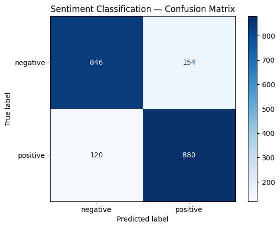

Error Analysis: Where Does the Model Fail?¶

Numbers tell us how much the model gets wrong. Error analysis tells us why. Let’s look at some misclassified reviews:

# Find misclassified examples
errors = []
for text, true, pred in zip(test_texts_small, test_labels_small, preds):
    if true != pred:
        errors.append((text, true, pred))

print(f"Total errors: {len(errors)} out of {len(test_texts_small)} ({len(errors)/len(test_texts_small):.1%})")
print("\n--- Sample misclassifications ---\n")
for text, true, pred in errors[:3]:
    true_label = label_names[true]
    pred_label = label_names[pred]
    print(f"TRUE: {true_label} | PREDICTED: {pred_label}")
    print(f"  {text[:200]}...")
    print()

Total errors: 274 out of 2000 (13.7%)

--- Sample misclassifications ---

TRUE: negative | PREDICTED: positive
  Teenager Tamara (Jenna Dewan) has it rough. She's ridiculed by all the popular "kids" for being shy, bookish, frumpy and because of her interest in witchcraft. All of the football players and cheerlea...

TRUE: negative | PREDICTED: positive
  Intended as light entertainment, this film is indeed successful as such during its first half, but then succumbs to a rapidly foundering script that drops it down. Harry (Judd Nelson), a "reformed" bu...

TRUE: positive | PREDICTED: negative
  It's really too bad that nobody knows about this movie. I think if it were just spruced up a little and if it weren't so low-budget, I think one of the major film companies might have wanted to take i...

Common failure patterns in sentiment analysis:

Negation: “not bad” contains “bad” but is positive
Sarcasm: “Oh great, another superhero movie” is negative despite “great”
Mixed sentiment: “the acting was great but the plot was terrible”
Subtle tone: reviews that use understated language

These are exactly the limitations of bag-of-words models — they can’t handle complex linguistic phenomena. Spoiler alert: this is what motivates the neural approaches we’ll study in Week 5 and beyond.

Exercise 4.6: Evaluation Deep Dive

Using the IMDB test predictions:

Compute precision, recall, and F1 for each class separately. Which class is easier to classify?
Find 3 false positives (predicted positive, actually negative) and 3 false negatives (predicted negative, actually positive). For each, can you identify why the classifier was fooled?
Suppose this classifier was being used to filter product reviews for a company dashboard, and the company only wants to see genuinely positive reviews. Should they optimize for precision or recall on the positive class? Explain.

# Starter code
from sklearn.metrics import precision_recall_fscore_support

# TODO: compute per-class precision, recall, F1
# HINT: precision_recall_fscore_support(test_labels_small, preds, average=None)

# TODO: find and examine false positives and false negatives
# HINT: filter errors list by (true, pred) values

Wrap-Up¶

Key Takeaways¶

Key Takeaways

Text classification maps documents to discrete categories — one of the most practical and widely-used NLP tasks
Naive Bayes uses Bayes’ theorem with a conditional independence assumption to classify efficiently; it’s a strong baseline especially with limited training data
Logistic Regression directly learns feature weights, offering good accuracy and interpretable coefficients that reveal which words drive predictions
Feature engineering matters: n-grams capture word context (especially negation), and TF-IDF weighting focuses on distinctive vocabulary
Scikit-learn Pipelines chain vectorization and classification into reproducible, leak-free workflows
SpaCy’s TextCategorizer integrates classification into the familiar SpaCy pipeline, making it easy to combine with tokenization, NER, and other components
Accuracy alone is misleading for imbalanced classes — always examine precision, recall, F1, and the confusion matrix to understand where and why a classifier fails

What’s Next¶

In the next lecture, we’ll move from classifying whole documents to labeling individual tokens within a document. Named entity recognition (NER) and part-of-speech tagging (POS tagging) are sequence labeling tasks — they require the model to make a decision for every token, not just one decision per document. We’ll use SpaCy’s built-in models and learn how to train custom NER models on domain-specific data.