Lab — Classify and Cluster
CAP-6640: Computational Understanding of Natural Language
Spencer Lyon
Prerequisites
L04.01: Text Classification (Naive Bayes, Logistic Regression, Scikit-learn pipelines, evaluation metrics)
L04.02: Sequence Labeling (NER, POS tagging, BIO scheme, SpaCy training)
Week 3: Text representations (TF-IDF, bag of words, word embeddings)
Outcomes
Build a complete sentiment classification pipeline from data loading through evaluation
Compare Naive Bayes, SVM, and Logistic Regression on the same dataset and interpret the differences
Perform systematic error analysis to identify classifier failure patterns
Apply K-means clustering to discover groupings in unlabeled text
Use LDA topic modeling to find latent themes in a document collection
References
J&M Chapter 4: Logistic Regression and Text Classification (download)
J&M Chapter 17: Sequence Labeling for Parts of Speech and Named Entities (download)
Lab Overview
This lab brings together everything from Week 4. We’ve built classifiers, labeled sequences, and evaluated models — now it’s time to put these skills into a cohesive workflow.
We’ll work through four scenarios:
Algorithm Showdown — Train and compare three classifiers on the same sentiment task
Error Analysis — Dig into why classifiers fail, not just how often
Unsupervised Exploration — Discover structure in text without labels using clustering and topic modeling
NER Under the Microscope — Stress-test entity recognition across domains
Each scenario builds on the lectures from this week. By the end, you’ll have hands-on experience with the full pipeline from raw text to actionable insights — both supervised and unsupervised.
Scenario 1: The Algorithm Showdown
In L04.01, we built sentiment classifiers with Naive Bayes and Logistic Regression. But how do they compare to each other — and to an SVM? Let’s find out with a head-to-head comparison on the IMDB dataset.
Loading and Preparing the Data
from datasets import load_dataset  # uv add datasets

# Load IMDB dataset
dataset = load_dataset("imdb")

# Shuffle — IMDB is sorted by label
dataset["train"] = dataset["train"].shuffle(seed=42)
dataset["test"] = dataset["test"].shuffle(seed=42)

# Use subsets for faster iteration
train_texts = dataset["train"]["text"][:5000]
train_labels = dataset["train"]["label"][:5000]
test_texts = dataset["test"]["text"][:2000]
test_labels = dataset["test"]["label"][:2000]

print(f"Training: {len(train_texts):,} reviews")
print(f"Test:     {len(test_texts):,} reviews")
print(f"Balance:  {sum(train_labels)} positive, {len(train_labels) - sum(train_labels)} negative")
Warning: You are sending unauthenticated requests to the HF Hub. Please set a HF_TOKEN to enable higher rate limits and faster downloads.
Training: 5,000 reviews
Test:     2,000 reviews
Balance:  2506 positive, 2494 negative
The Three Contenders
We’ll use the same TF-IDF representation for all three classifiers so the comparison is fair — only the learning algorithm changes:
import time
from sklearn.pipeline import Pipeline
from sklearn.feature_extraction.text import TfidfVectorizer
from sklearn.naive_bayes import MultinomialNB
from sklearn.linear_model import LogisticRegression
from sklearn.svm import LinearSVC
from sklearn.metrics import accuracy_score, f1_score

classifiers = {
    "Naive Bayes": MultinomialNB(),
    "Logistic Regression": LogisticRegression(max_iter=1000),
    "SVM (Linear)": LinearSVC(max_iter=1000),
}

results = {}

for name, clf in classifiers.items():
    pipe = Pipeline([
        ("tfidf", TfidfVectorizer(max_features=20000, ngram_range=(1, 2))),
        ("clf", clf),
    ])

    start = time.time()
    pipe.fit(train_texts, train_labels)
    train_time = time.time() - start

    preds = pipe.predict(test_texts)
    acc = accuracy_score(test_labels, preds)
    f1 = f1_score(test_labels, preds, average="weighted")

    results[name] = {
        "pipeline": pipe,
        "predictions": preds,
        "accuracy": acc,
        "f1": f1,
        "train_time": train_time,
    }
    print(f"{name:25s}  accuracy={acc:.3f}  F1={f1:.3f}  time={train_time:.2f}s")
Naive Bayes accuracy=0.856 F1=0.855 time=2.19s
Logistic Regression accuracy=0.863 F1=0.863 time=2.24s
SVM (Linear) accuracy=0.871 F1=0.870 time=2.28s
Visualizing the Results
import matplotlib.pyplot as plt
import numpy as np

names = list(results.keys())
accs = [results[n]["accuracy"] for n in names]
f1s = [results[n]["f1"] for n in names]
times = [results[n]["train_time"] for n in names]

fig, axes = plt.subplots(1, 2, figsize=(10, 4))

# Accuracy and F1
x = np.arange(len(names))
width = 0.35
axes[0].bar(x - width / 2, accs, width, label="Accuracy", color="#4C72B0")
axes[0].bar(x + width / 2, f1s, width, label="F1 (weighted)", color="#55A868")
axes[0].set_xticks(x)
axes[0].set_xticklabels(names, fontsize=9)
axes[0].set_ylim(0.8, 0.92)
axes[0].set_ylabel("Score")
axes[0].set_title("Classification Performance")
axes[0].legend()

# Training time
axes[1].bar(names, times, color="#C44E52")
axes[1].set_ylabel("Seconds")
axes[1].set_title("Training Time")

plt.tight_layout()
plt.show()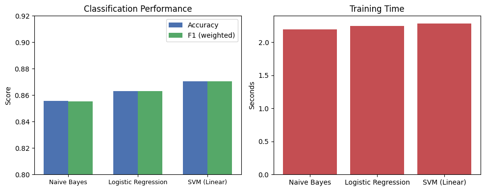
Interpreting the Results
The differences are small but instructive:
Naive Bayes is fast and simple, but its independence assumption limits accuracy — correlated features (like bigrams) get double-counted.
Logistic Regression learns feature weights directly, handling correlations better. It’s a strong default for text classification.
SVM (Linear) finds the maximum-margin decision boundary. It often edges out Logistic Regression slightly, especially with high-dimensional sparse features like TF-IDF.
All three use the same TF-IDF features, so the differences come entirely from how each algorithm uses those features to draw decision boundaries.
What Do the Feature Weights Tell Us?
Logistic Regression gives us interpretable weights — let’s look at what drives its decisions:
import pandas as pd

# Get the Logistic Regression pipeline
lr_pipe = results["Logistic Regression"]["pipeline"]
features = lr_pipe["tfidf"].get_feature_names_out()
weights = lr_pipe["clf"].coef_[0]

weight_df = pd.DataFrame({"feature": features, "weight": weights})
weight_df = weight_df.sort_values("weight", ascending=False)

print("Top 10 features for POSITIVE sentiment:")
print(weight_df.head(10).to_string(index=False))
print("\nTop 10 features for NEGATIVE sentiment:")
print(weight_df.tail(10).to_string(index=False))
Top 10 features for POSITIVE sentiment:
feature weight
great 4.308561
best 2.639015
very 2.361742
the best 2.355279
excellent 2.319303
love 2.318560
and 2.002370
amazing 1.946124
well 1.907251
wonderful 1.903622
Top 10 features for NEGATIVE sentiment:
feature weight
nothing -2.310162
boring -2.320332
just -2.355827
awful -2.374511
waste -2.438897
poor -2.534181
the worst -2.658157
no -2.778859
worst -3.387703
bad -4.818013
Notice the bigrams: features like “not worth” or “not good” might appear among the negative indicators, while “well worth” or “great film” appear among the positive. This is exactly why n-grams matter — they capture negation and multi-word expressions that unigrams miss.
Scenario 2: Error Analysis Deep Dive
Accuracy numbers tell us how often a model gets things wrong. Error analysis tells us why. Let’s dig into the misclassifications from our best classifier.
Finding the Errors
# Use the SVM predictions (our best performer)
best_preds = results["SVM (Linear)"]["predictions"]
label_names = ["negative", "positive"]

errors = []
for text, true_l, pred_l in zip(test_texts, test_labels, best_preds):
    if true_l != pred_l:
        errors.append({"text": text, "true": label_names[true_l], "predicted": label_names[pred_l]})

print(f"Errors: {len(errors)} out of {len(test_texts)} ({len(errors) / len(test_texts):.1%})")
Errors: 259 out of 2000 (13.0%)
Examining Error Cases
Let’s look at some misclassified reviews to find patterns:
# False positives: predicted positive, actually negative
false_positives = [e for e in errors if e["true"] == "negative"]
print(f"=== False Positives ({len(false_positives)} total) ===")
print(f"(Predicted POSITIVE, actually NEGATIVE)\n")
for e in false_positives[:3]:
    print(f"  {e['text'][:200]}...")
    print()

# False negatives: predicted negative, actually positive
false_negatives = [e for e in errors if e["true"] == "positive"]
print(f"=== False Negatives ({len(false_negatives)} total) ===")
print(f"(Predicted NEGATIVE, actually POSITIVE)\n")
for e in false_negatives[:3]:
    print(f"  {e['text'][:200]}...")
    print()
=== False Positives (137 total) ===
(Predicted POSITIVE, actually NEGATIVE)
This movie was so frustrating. Everything seemed energetic and I was totally prepared to have a good time. I at least thought I'd be able to stand it. But, I was wrong. First, the weird looping? It wa...
Porn legend Gregory Dark directs this cheesy horror flick that has Glen Jacobs (Kane from WWF/WWE/ whatever it calls itself nowadays) in his cinematic debut. He plays Jacob Goodknight, a blind serial ...
A not so good action thriller because it unsuccessfully trends the same water as early Steven Seagal films because there is not a very good set piece. Steven Seagal plays the same kind of character th...
=== False Negatives (122 total) ===
(Predicted NEGATIVE, actually POSITIVE)
This is a really sad, and touching movie! It deals with the subject of child abuse. It's really sad, but mostly a true story, because it happens everyday. Elijah Wood and Joseph Mazzello play the two ...
It's really too bad that nobody knows about this movie. I think if it were just spruced up a little and if it weren't so low-budget, I think one of the major film companies might have wanted to take i...
At first I didn't think that the performance by Lauren Ambrose was anything but flaky, but as her character developed the portrayal made more sense. Amy Madigan seemed too terse for her role and didn'...
Categorizing Errors
As we look at these examples, common patterns emerge. Let’s try to categorize them:
# Let's check for some telltale patterns in misclassified reviews
negation_words = {"not", "no", "never", "neither", "barely", "hardly", "doesn't", "didn't", "wasn't", "won't", "can't", "couldn't", "shouldn't"}
contrast_words = {"but", "however", "although", "though", "yet", "despite", "except"}

for category, keywords in [("Negation", negation_words), ("Contrast/mixed", contrast_words)]:
    count = 0
    for e in errors:
        words = set(e["text"].lower().split())
        if words & keywords:
            count += 1
    print(f"Errors containing {category.lower()} words: {count}/{len(errors)} ({count / len(errors):.0%})")
Errors containing negation words: 222/259 (86%)
Errors containing contrast/mixed words: 203/259 (78%)
These numbers are informative: reviews with negation or contrast words are harder because bag-of-words models struggle with context. “Not bad” contains the word “bad” but expresses a positive (or at least neutral) sentiment. A review that says “the acting was brilliant but the plot was terrible” has signals pointing both ways.
Per-Class Breakdown
from sklearn.metrics import classification_report, confusion_matrix, ConfusionMatrixDisplay

print(classification_report(test_labels, best_preds, target_names=label_names))
precision recall f1-score support
negative 0.88 0.86 0.87 1000
positive 0.87 0.88 0.87 1000
accuracy 0.87 2000
macro avg 0.87 0.87 0.87 2000
weighted avg 0.87 0.87 0.87 2000
cm = confusion_matrix(test_labels, best_preds)
disp = ConfusionMatrixDisplay(confusion_matrix=cm, display_labels=label_names)
disp.plot(cmap="Blues")
plt.title("SVM Sentiment Classifier — Confusion Matrix")
plt.show()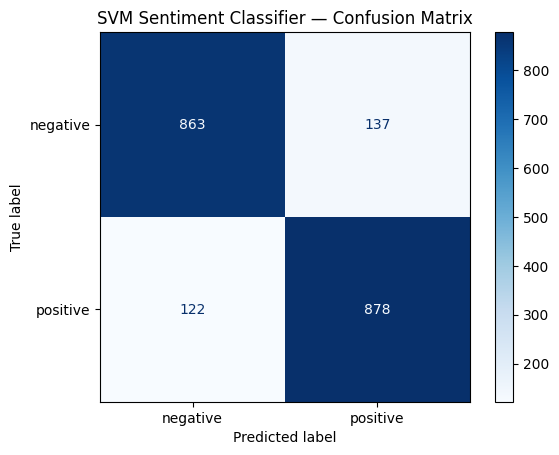
Scenario 3: Unsupervised Text Exploration
So far this week, everything has been supervised — we had labels and trained models to predict them. But what if you have a pile of documents with no labels? Can we still discover meaningful structure?
This is where unsupervised methods come in. We’ll explore two complementary approaches:
K-means clustering: group documents by vector similarity
LDA topic modeling: discover latent themes across a collection
Setting Up the Data
We’ll use the 20 Newsgroups dataset — a classic collection of newsgroup posts organized by topic. We’ll pick four categories to keep things interpretable:
from sklearn.datasets import fetch_20newsgroups

categories = ["rec.sport.baseball", "sci.space", "comp.graphics", "talk.politics.guns"]

newsgroups = fetch_20newsgroups(
    subset="train",
    categories=categories,
    remove=("headers", "footers", "quotes"),  # Strip metadata to focus on content
)

print(f"Loaded {len(newsgroups.data):,} documents")
print(f"Categories: {newsgroups.target_names}")
print(f"\nSample document (first 200 chars):")
print(f"  {newsgroups.data[0][:200]}...")
print(f"  Category: {newsgroups.target_names[newsgroups.target[0]]}")
Loaded 2,320 documents
Categories: ['comp.graphics', 'rec.sport.baseball', 'sci.space', 'talk.politics.guns']
Sample document (first 200 chars):
What about guns with non-lethal bullets, like rubber or plastic bullets. Would
those work very well in stopping an attack?...
Category: talk.politics.guns
K-Means Clustering
K-means is conceptually simple: represent each document as a TF-IDF vector, then partition documents into K groups by minimizing the distance from each document to its cluster centroid.
from sklearn.feature_extraction.text import TfidfVectorizer
from sklearn.cluster import KMeans

# Vectorize
vectorizer = TfidfVectorizer(max_features=5000, stop_words="english")
X_tfidf = vectorizer.fit_transform(newsgroups.data)
print(f"TF-IDF matrix: {X_tfidf.shape[0]} documents × {X_tfidf.shape[1]} features")

# Cluster
km = KMeans(n_clusters=4, random_state=42, n_init=10)
km.fit(X_tfidf)

# What are the clusters about? Look at the top terms near each centroid
feature_names = vectorizer.get_feature_names_out()

print("\n--- Top terms per cluster ---")
for i in range(4):
    top_indices = km.cluster_centers_[i].argsort()[-10:][::-1]
    top_terms = [feature_names[j] for j in top_indices]
    print(f"  Cluster {i}: {', '.join(top_terms)}")
TF-IDF matrix: 2320 documents × 5000 features
--- Top terms per cluster ---
Cluster 0: year, team, game, games, runs, hit, baseball, pitching, good, think
Cluster 1: space, just, like, nasa, think, time, don, edu, com, know
Cluster 2: gun, people, don, guns, right, government, think, just, fbi, law
Cluster 3: thanks, graphics, files, know, file, program, image, does, mail, looking
The top terms give a clear signal: one cluster talks about “space” and “nasa”, another about “game” and “team”, another about “gun” and “government”, and another about “image” and “graphics.” Without ever seeing a label, K-means has discovered the underlying topics.
How Good Are the Clusters?
Since we do have the true labels, we can check how well the clusters align with the actual categories:
import numpy as np
from collections import Counter

print("--- Cluster composition ---")
for i in range(4):
    cluster_mask = km.labels_ == i
    true_labels = np.array(newsgroups.target)[cluster_mask]
    label_counts = Counter(true_labels)
    total = sum(label_counts.values())
    print(f"\nCluster {i} ({total} docs):")
    for label_id, count in label_counts.most_common():
        pct = count / total * 100
        print(f"  {newsgroups.target_names[label_id]:30s} {count:4d} ({pct:.0f}%)")
--- Cluster composition ---
Cluster 0 (334 docs):
rec.sport.baseball 331 (99%)
sci.space 2 (1%)
comp.graphics 1 (0%)
Cluster 1 (1117 docs):
sci.space 539 (48%)
rec.sport.baseball 236 (21%)
comp.graphics 173 (15%)
talk.politics.guns 169 (15%)
Cluster 2 (417 docs):
talk.politics.guns 374 (90%)
sci.space 29 (7%)
rec.sport.baseball 8 (2%)
comp.graphics 6 (1%)
Cluster 3 (452 docs):
comp.graphics 404 (89%)
sci.space 23 (5%)
rec.sport.baseball 22 (5%)
talk.politics.guns 3 (1%)
Choosing K: The Elbow Method
We picked K=4 because we knew there were 4 categories. In practice, you won’t know the right number of clusters. The elbow method plots inertia (within-cluster sum of squared distances) against K and looks for a “bend”:
inertias = []
K_range = range(2, 9)

for k in K_range:
    km_temp = KMeans(n_clusters=k, random_state=42, n_init=10)
    km_temp.fit(X_tfidf)
    inertias.append(km_temp.inertia_)

plt.figure(figsize=(7, 4))
plt.plot(list(K_range), inertias, "o-", color="#4C72B0")
plt.xlabel("Number of clusters (K)")
plt.ylabel("Inertia")
plt.title("Elbow Method for K-Means")
plt.xticks(list(K_range))
plt.grid(alpha=0.3)
plt.show()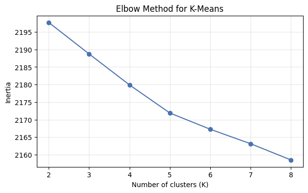
The elbow isn’t always sharp, but you can often see the curve flattening out — adding more clusters beyond that point gives diminishing returns.
LDA Topic Modeling
K-means assigns each document to exactly one cluster. Latent Dirichlet Allocation (LDA) takes a different view: each document is a mixture of topics, and each topic is a distribution over words.
Think of it this way: a news article about a sports team’s stadium deal might be 60% “sports” and 40% “business.” K-means forces a hard assignment; LDA allows soft, overlapping membership.
from sklearn.feature_extraction.text import CountVectorizer
from sklearn.decomposition import LatentDirichletAllocation

# LDA works with raw counts, not TF-IDF
count_vec = CountVectorizer(max_features=5000, stop_words="english")
X_counts = count_vec.fit_transform(newsgroups.data)

# Fit LDA with 4 topics
lda = LatentDirichletAllocation(n_components=4, random_state=42, max_iter=10)
lda.fit(X_counts)

# Show top words per topic
lda_feature_names = count_vec.get_feature_names_out()

print("--- LDA Topics ---")
for i, topic in enumerate(lda.components_):
    top_indices = topic.argsort()[-10:][::-1]
    top_terms = [lda_feature_names[j] for j in top_indices]
    print(f"  Topic {i}: {', '.join(top_terms)}")
--- LDA Topics ---
Topic 0: space, nasa, launch, satellite, shuttle, earth, orbit, lunar, new, data
Topic 1: year, just, think, don, good, like, time, game, better, team
Topic 2: image, edu, graphics, file, software, data, jpeg, ftp, images, files
Topic 3: gun, people, guns, don, file, firearms, right, law, 00, like
Comparing K-Means and LDA
Both found meaningful structure, but they work differently:
| Aspect | K-Means | LDA |
|---|---|---|
| Assignment | Hard — each doc in one cluster | Soft — each doc is a mix of topics |
| Input | TF-IDF vectors | Raw word counts |
| Approach | Distance-based (geometric) | Probabilistic (generative model) |
| Interpretability | Cluster centroids → top terms | Topic distributions → top terms |
| Overlap | No | Yes — a document can be about multiple topics |
Let’s see LDA’s soft assignments in action:
# Transform a few documents to see their topic mixtures
topic_distributions = lda.transform(X_counts[:5])

for i in range(5):
    print(f"Document {i} (true: {newsgroups.target_names[newsgroups.target[i]]})")
    for j in range(4):
        bar = "█" * int(topic_distributions[i][j] * 30)
        print(f"  Topic {j}: {topic_distributions[i][j]:.2f} {bar}")
    print()
Document 0 (true: talk.politics.guns)
Topic 0: 0.02
Topic 1: 0.02
Topic 2: 0.02
Topic 3: 0.93 ███████████████████████████
Document 1 (true: rec.sport.baseball)
Topic 0: 0.03
Topic 1: 0.76 ██████████████████████
Topic 2: 0.03
Topic 3: 0.19 █████
Document 2 (true: sci.space)
Topic 0: 0.01
Topic 1: 0.63 ██████████████████
Topic 2: 0.34 ██████████
Topic 3: 0.01
Document 3 (true: talk.politics.guns)
Topic 0: 0.00
Topic 1: 0.56 ████████████████
Topic 2: 0.00
Topic 3: 0.44 █████████████
Document 4 (true: sci.space)
Topic 0: 0.63 ██████████████████
Topic 1: 0.36 ██████████
Topic 2: 0.01
Topic 3: 0.01
Notice how some documents are strongly associated with a single topic, while others have a more mixed profile. This flexibility is one of LDA’s main advantages over hard clustering.
Scenario 4: NER Under the Microscope
In L04.02 we trained a custom NER model and noted that SpaCy’s built-in model struggles on domain-specific text. Let’s put that to a systematic test.
Cross-Domain NER Evaluation
import spacy

nlp = spacy.load("en_core_web_sm")

domain_texts = {
    "News": (
        "President Biden met with Chancellor Scholz in Berlin on Monday "
        "to discuss a $50 billion NATO defense package."
    ),
    "Medical": (
        "Patient was prescribed Metformin 500mg and Lisinopril 10mg. "
        "Dr. Sarah Chen at Mayo Clinic recommends follow-up in March."
    ),
    "Social media": (
        "omg just saw Beyonce at Coachella in Indio CA!!! "
        "she was wearing Gucci and arrived in a Tesla lol #iconic"
    ),
    "Legal": (
        "The defendant, John Smith, is charged under Section 18 U.S.C. 1343. "
        "Judge Martinez of the Southern District of New York will preside."
    ),
    "Scientific": (
        "Researchers at Stanford University used the CRISPR-Cas9 system "
        "to modify the BRCA1 gene in a study published in Nature Genetics."
    ),
}

for domain, text in domain_texts.items():
    doc = nlp(text)
    ents = [(ent.text, ent.label_) for ent in doc.ents]
    print(f"{domain}:")
    for ent_text, ent_label in ents:
        print(f"  {ent_text:30s} → {ent_label}")
    if not ents:
        print("  (no entities detected)")
    print()
News:
Biden → PERSON
Berlin → GPE
Monday → DATE
$50 billion → MONEY
NATO → ORG
Medical:
500 → CARDINAL
Lisinopril 10 → LAW
Sarah Chen → PERSON
Mayo Clinic → ORG
March → DATE
Social media:
Gucci → PERSON
Tesla → ORG
# → CARDINAL
Legal:
John Smith → PERSON
Section 18 U.S.C. → LAW
1343 → DATE
Martinez → PERSON
the Southern District → LOC
New York → GPE
Scientific:
Stanford University → ORG
BRCA1 → NORP
Nature Genetics → WORK_OF_ART
Categorizing NER Errors
Let’s annotate the expected entities and compare systematically:
# Gold annotations: (text, expected_entities)
gold_annotations = {
    "News": [
        ("Biden", "PERSON"), ("Scholz", "PERSON"), ("Berlin", "GPE"),
        ("Monday", "DATE"), ("$50 billion", "MONEY"), ("NATO", "ORG"),
    ],
    "Medical": [
        ("Metformin", "PRODUCT"), ("Lisinopril", "PRODUCT"),
        ("Sarah Chen", "PERSON"), ("Mayo Clinic", "ORG"), ("March", "DATE"),
    ],
    "Social media": [
        ("Beyonce", "PERSON"), ("Coachella", "EVENT"), ("Indio", "GPE"),
        ("CA", "GPE"), ("Gucci", "ORG"), ("Tesla", "ORG"),
    ],
    "Legal": [
        ("John Smith", "PERSON"), ("Martinez", "PERSON"),
        ("Southern District of New York", "ORG"),
    ],
    "Scientific": [
        ("Stanford University", "ORG"), ("Nature Genetics", "ORG"),
    ],
}

error_types = {"boundary": 0, "type_confusion": 0, "missed": 0, "spurious": 0}

for domain, text in domain_texts.items():
    doc = nlp(text)
    pred = {(ent.text, ent.label_) for ent in doc.ents}
    gold = set(gold_annotations[domain])

    pred_texts = {ent_text for ent_text, _ in pred}
    gold_texts = {ent_text for ent_text, _ in gold}

    for ent_text, ent_label in gold:
        if (ent_text, ent_label) in pred:
            continue  # Correct
        elif ent_text in pred_texts:
            error_types["type_confusion"] += 1
        else:
            # Check for partial overlap (boundary error)
            found_partial = False
            for p_text, _ in pred:
                if ent_text in p_text or p_text in ent_text:
                    error_types["boundary"] += 1
                    found_partial = True
                    break
            if not found_partial:
                error_types["missed"] += 1

    for ent_text, ent_label in pred:
        if ent_text not in gold_texts:
            # Check if it's a boundary variant
            found_partial = False
            for g_text, _ in gold:
                if ent_text in g_text or g_text in ent_text:
                    found_partial = True
                    break
            if not found_partial:
                error_types["spurious"] += 1

print("--- NER Error Summary Across Domains ---")
for err_type, count in error_types.items():
    print(f"  {err_type:20s}: {count}")
--- NER Error Summary Across Domains ---
boundary : 2
type_confusion : 2
missed : 6
spurious : 6
The pattern is clear: models trained on well-edited news text struggle when confronted with medical jargon, social media conventions, or specialized legal language. This is a fundamental challenge in NLP — domain shift means a model’s performance on the data it was trained on doesn’t predict its performance in a new domain.
Wrap-Up
Key Takeaways
What’s Next
We’ve now built a solid foundation in classical NLP — tokenization, text representation, classification, sequence labeling, and unsupervised analysis. But we’ve also seen the limits: bag-of-words models can’t handle negation, sarcasm, or long-range context. In Week 5, we’ll break through these limitations by moving to neural networks for NLP. We’ll build feed-forward and recurrent (LSTM) text classifiers in PyTorch, discovering how neural approaches learn representations directly from data instead of relying on hand-crafted features like TF-IDF.