Feed-Forward Networks for Text
CAP-6640: Computational Understanding of Natural Language
Spencer Lyon
Prerequisites
L04.01–03: Text classification, evaluation metrics (precision, recall, F1 score)
L03.01–02: Text representations (TF-IDF, word embeddings)
Basic linear algebra (vectors, matrices, dot products)
Outcomes
Explain the core building blocks of a neural network: neurons, layers, activation functions, and loss functions
Describe how text is transformed into input representations suitable for neural networks
Implement a feed-forward network text classifier in PyTorch using
nn.ModuleTrain, evaluate, and diagnose a neural classifier on real movie review data
Apply regularization techniques (dropout) to combat overfitting
References
Why Go Neural?
Last week we built text classifiers with Naive Bayes, Logistic Regression, and SVMs (Week 4). They worked surprisingly well — so why do we need anything more complex?
Here’s the catch: those classical models depend heavily on the features we engineer. We had to choose between bag of words, TF-IDF weighting, n-grams, and so on. Every choice baked in assumptions about what matters in the text. If we got the features wrong, the model had no way to recover.
Neural networks flip this around. Instead of hand-crafting features, we give the network raw-ish inputs (like word embeddings) and let it learn what features matter for the task. The network discovers its own internal representations — ones that might be more useful than anything we’d design by hand.
There are three big reasons to go neural:
Learned features: The network extracts patterns we might never think to engineer
Compositionality: Deep networks build complex features from simple ones — layer by layer
Foundation for what’s next: RNNs, LSTMs, and Transformers (weeks 5–7) all build on the ideas we’ll learn today
We’ll start with the simplest neural architecture — the feed-forward network — and use it to build a sentiment classifier on real movie reviews. By the end of this lecture, you’ll have a working PyTorch model trained on IMDB data.
Neural Network Fundamentals
The Neuron: A Weighted Vote
The building block of every neural network is the neuron (or unit). A neuron does three things:
Takes a set of inputs
Computes a weighted sum:
Passes the result through an activation function:
The weights determine how much each input matters. The bias shifts the decision boundary. And the activation function introduces non-linearity — without it, stacking layers would be pointless (a composition of linear functions is still linear).
Let’s see this in code:
import numpy as np

# A single neuron with 3 inputs
inputs = np.array([0.8, 0.2, -0.5])
weights = np.array([0.4, 0.9, -0.3])
bias = 0.1

# Step 1: Weighted sum
z = np.dot(inputs, weights) + bias
print(f"Inputs:       {inputs}")
print(f"Weights:      {weights}")
print(f"Weighted sum: z = {z:.3f}")

# Step 2: ReLU activation: max(0, z)
a = max(0, z)
print(f"After ReLU:   a = {a:.3f}")
Inputs: [ 0.8 0.2 -0.5]
Weights: [ 0.4 0.9 -0.3]
Weighted sum: z = 0.750
After ReLU: a = 0.750
That’s it — one neuron is just a dot product, a bias, and a non-linearity. The magic happens when we stack many of these together — but getting there requires a shift from vectors to matrices, so let’s take that step carefully.
From One Neuron to a Layer (Vectors → Matrices)
Our single neuron takes an input vector and produces a single scalar output:
But one neuron can only learn one feature. What if we want neurons, each looking at the same input but learning different patterns? Neuron 1 has weights , neuron 2 has , and so on. We could write each one separately:
That’s tedious. But notice: each is a dot product of a weight row with the same input vector. If we stack all weight vectors into a matrix (where row is ) and all biases into a vector , every neuron’s output can be computed in one shot:
Here and , so — one entry per neuron. This collection of neurons all operating on the same input is called a layer.
# From 1 neuron to a layer of 4 neurons
x = np.array([0.8, 0.2, -0.5])   # Same 3 inputs as before

# 4 neurons, each with its own weights (4 x 3 weight matrix)
W = np.array([
    [ 0.4,  0.9, -0.3],   # neuron 1: same weights as our earlier example
    [-0.2,  0.5,  0.1],   # neuron 2: different pattern
    [ 0.7, -0.1,  0.6],   # neuron 3: yet another pattern
    [ 0.0,  0.3, -0.8],   # neuron 4: and another
])
b = np.array([0.1, -0.1, 0.0, 0.2])

z = W @ x + b  # Matrix-vector multiply + bias
print(f"Input x shape:  {x.shape}  (n=3 features)")
print(f"Weight W shape: {W.shape}  (m=4 neurons, n=3 inputs)")
print(f"Output z shape: {z.shape}  (m=4 neuron outputs)")
print(f"z = {z}")
Input x shape: (3,) (n=3 features)
Weight W shape: (4, 3) (m=4 neurons, n=3 inputs)
Output z shape: (4,) (m=4 neuron outputs)
z = [ 0.75 -0.21 0.24 0.66]
Now, what about handling multiple observations at the same time? In training we don’t feed one example at a time — we process a batch of examples for efficiency. If each example is a row of a matrix , we can run the entire batch through the layer in a single operation:
Here each row of holds the outputs of all neurons for one example. The matrix multiply handles everything in parallel — every example paired with every neuron, all at once.
# A batch of 3 observations, each with 3 features
X_batch = np.array([
    [ 0.8,  0.2, -0.5],   # observation 1 (same as our single example)
    [-0.1,  0.4,  0.3],   # observation 2
    [ 0.6, -0.3,  0.9],   # observation 3
])

Z_batch = X_batch @ W.T + b  # (3 x 3) @ (3 x 4) + (4,) = (3 x 4)
print(f"Batch X shape:  {X_batch.shape}  (B=3 examples, n=3 features)")
print(f"Output Z shape: {Z_batch.shape}  (B=3 examples, m=4 neurons)")
print(f"\nZ =\n{Z_batch.round(3)}")
print(f"\nRow 0 matches our single-example result: {np.allclose(Z_batch[0], z)}")
Batch X shape: (3, 3) (B=3 examples, n=3 features)
Output Z shape: (3, 4) (B=3 examples, m=4 neurons)
Z =
[[ 0.75 -0.21 0.24 0.66]
[ 0.33 0.15 0.07 0.08]
[-0.2 -0.28 0.99 -0.61]]
Row 0 matches our single-example result: True
To summarize the dimensional progression:
| Step | Operation | Input | Output |
|---|---|---|---|
| 1 neuron, 1 observation | vector | scalar | |
| neurons, 1 observation | vector | vector | |
| neurons, observations | matrix | matrix |
This is the key mental model: a layer is just a matrix multiply that applies many neurons in parallel, and batching adds one more dimension so many observations are processed simultaneously. Every subsequent formula in this lecture uses this matrix notation, and now you know exactly what it means — many neurons times many examples, computed all at once.
Activation Functions: The Non-Linear Ingredient
Why do we need activation functions? To see why, let’s focus on a single observation to keep the algebra clean. (Everything we show here applies row-by-row across a batch — the linearity argument is the same whether we write for one example or for a batch.)
Consider what happens without activation functions. If each layer just computes , then stacking two layers gives us:
That’s just another linear transformation — two layers collapse into one. No matter how many layers we stack, we’d never escape linearity. Activation functions break this limitation by applying a non-linear function element-wise between layers.
Here are the three you’ll see most often:
import matplotlib.pyplot as plt

x = np.linspace(-5, 5, 200)

fig, axes = plt.subplots(1, 3, figsize=(12, 3))

# Sigmoid: squashes to (0, 1)
axes[0].plot(x, 1 / (1 + np.exp(-x)), linewidth=2)
axes[0].set_title("Sigmoid: $\\sigma(z) = 1/(1+e^{-z})$")
axes[0].set_ylim(-0.1, 1.1)

# Tanh: squashes to (-1, 1)
axes[1].plot(x, np.tanh(x), linewidth=2, color="orange")
axes[1].set_title("Tanh: $\\tanh(z)$")
axes[1].set_ylim(-1.3, 1.3)

# ReLU: max(0, z) — the modern default
axes[2].plot(x, np.maximum(0, x), linewidth=2, color="green")
axes[2].set_title("ReLU: $\\max(0, z)$")

for ax in axes:
    ax.axhline(0, color="gray", linewidth=0.5)
    ax.axvline(0, color="gray", linewidth=0.5)
    ax.grid(True, alpha=0.3)

plt.tight_layout()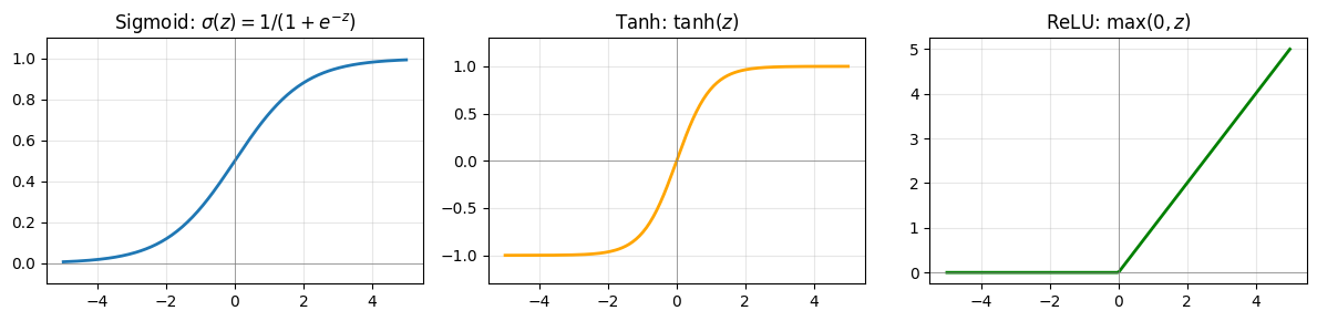
In practice:
ReLU is the default for hidden layers — it’s simple, fast, and works well
Sigmoid appears at the output for binary classification (outputs a probability between 0 and 1)
Softmax (a generalization of sigmoid) is used for multi-class outputs — it converts a vector of raw scores into probabilities that sum to 1
The Feed-Forward Architecture

Figure 1:A feed-forward network for text classification — words are embedded, averaged into a single vector, transformed through a hidden layer with ReLU activation, and mapped to class probabilities.
A feed-forward network arranges neurons into layers where information flows in one direction: input → hidden → output. Using our batch notation (where each row of a matrix is one example):
Each layer transforms its input through a linear operation (weights + bias) followed by a non-linear activation or . The hidden layer learns an internal representation of the input — a new set of features that are useful for the task. The output layer maps this representation to predictions. (For a single example, replace each matrix with its corresponding vector: , , , and the transposes become plain matrix-vector products.)
Why is depth useful? Each layer builds on the features learned by the previous one. The first layer might detect simple patterns (presence of certain words), while the second combines these into higher-level concepts (sentiment-bearing phrases). This hierarchical feature learning is the fundamental advantage of deep networks.
From Text to Tensors
Neural networks operate on numbers — specifically, tensors (multi-dimensional arrays). So how do we feed text into a neural network?
We already know the answer from Week 3: embeddings. Recall that a word embedding maps each word to a dense vector that captures its meaning. The question is how to go from a sequence of word vectors to a single fixed-size vector that we can feed into our classifier.
The simplest approach is mean pooling — average all the word vectors in a document:
where is the embedding of word and is the number of words. This throws away word order (just like bag of words!), but it gives us a fixed-size vector regardless of document length.
We have two options for where the embeddings come from:
Pre-trained embeddings: Use vectors from Word2Vec, GloVe, etc. Good when training data is limited.
Learned embeddings: Initialize randomly and let the network learn them during training. This is what we’ll do — PyTorch’s
nn.Embeddingmakes it easy.
The full architecture for our text classifier looks like this:
Building a Neural Text Classifier
Time to build something real. We’ll create a feed-forward sentiment classifier for IMDB movie reviews using PyTorch.
Preparing the Data
import torch
import torch.nn as nn
from torch.utils.data import DataLoader, TensorDataset
from datasets import load_dataset
from collections import Counter

# Load IMDB (shuffle first — the dataset is sorted by label!)
dataset = load_dataset("imdb")
train_data = dataset["train"].shuffle(seed=42).select(range(5000))
test_data = dataset["test"].shuffle(seed=42).select(range(1000))

print(f"Training examples: {len(train_data)}")
print(f"Test examples:     {len(test_data)}")
print(f"\nSample review (first 200 chars):")
print(train_data[0]["text"][:200] + "...")
print(f"Label: {train_data[0]['label']} ({'positive' if train_data[0]['label'] == 1 else 'negative'})")
Training examples: 5000
Test examples: 1000
Sample review (first 200 chars):
There is no relation at all between Fortier and Profiler but the fact that both are police series about violent crimes. Profiler looks crispy, Fortier looks classic. Profiler plots are quite simple. F...
Label: 1 (positive)
We’re using a 5,000-example subset to keep training fast. In practice, you’d use the full 25,000.
Next, we need a vocabulary — a mapping from words to integer indices. The network doesn’t understand strings; it needs numbers.
def build_vocab(texts, max_vocab=10000):
    """Build a vocabulary mapping words to integer indices."""
    counter = Counter()
    for text in texts:
        counter.update(text.lower().split())

    # Reserve 0 for padding, 1 for unknown words
    vocab = {"<pad>": 0, "<unk>": 1}
    for word, _ in counter.most_common(max_vocab - 2):
        vocab[word] = len(vocab)
    return vocab

vocab = build_vocab(train_data["text"])
print(f"Vocabulary size: {len(vocab):,}")
print(f"Index of 'movie': {vocab.get('movie', 'not found')}")
print(f"Index of 'terrible': {vocab.get('terrible', 'not found')}")
Vocabulary size: 10,000
Index of 'movie': 20
Index of 'terrible': 550
Now we convert each review into a fixed-length sequence of integer indices:
def encode_texts(texts, vocab, max_len=256):
    """Convert texts to padded integer sequences."""
    encoded = []
    for text in texts:
        tokens = text.lower().split()[:max_len]  # Truncate long reviews
        indices = [vocab.get(t, vocab["<unk>"]) for t in tokens]
        indices += [vocab["<pad>"]] * (max_len - len(indices))  # Pad short ones
        encoded.append(indices)
    return torch.tensor(encoded)

X_train = encode_texts(train_data["text"], vocab)
y_train = torch.tensor(train_data["label"])
X_test = encode_texts(test_data["text"], vocab)
y_test = torch.tensor(test_data["label"])

print(f"Training tensor shape: {X_train.shape}")
print(f"Labels shape:          {y_train.shape}")
print(f"First review (first 10 indices): {X_train[0][:10].tolist()}")
Training tensor shape: torch.Size([5000, 256])
Labels shape: torch.Size([5000])
First review (first 10 indices): [52, 7, 63, 8099, 30, 34, 191, 1, 4, 1]
Defining the Model
Here’s our feed-forward classifier. PyTorch’s nn.Module gives us a clean way to define the architecture:
class FeedForwardClassifier(nn.Module):
    def __init__(self, vocab_size, embed_dim, hidden_dim, num_classes):
        super().__init__()
        self.embedding = nn.Embedding(vocab_size, embed_dim, padding_idx=0)
        self.fc1 = nn.Linear(embed_dim, hidden_dim)
        self.relu = nn.ReLU()
        self.fc2 = nn.Linear(hidden_dim, num_classes)

    def forward(self, x):
        # x shape: (batch_size, seq_len)
        embeds = self.embedding(x)             # (batch_size, seq_len, embed_dim)

        # Mean pooling: average word vectors, ignoring padding tokens
        mask = (x != 0).unsqueeze(-1).float()  # (batch_size, seq_len, 1)
        pooled = (embeds * mask).sum(dim=1) / mask.sum(dim=1).clamp(min=1)

        hidden = self.relu(self.fc1(pooled))   # (batch_size, hidden_dim)
        output = self.fc2(hidden)              # (batch_size, num_classes)
        return output

model = FeedForwardClassifier(
    vocab_size=len(vocab),
    embed_dim=64,
    hidden_dim=128,
    num_classes=2,
)
print(model)

total_params = sum(p.numel() for p in model.parameters())
print(f"\nTotal trainable parameters: {total_params:,}")
FeedForwardClassifier(
(embedding): Embedding(10000, 64, padding_idx=0)
(fc1): Linear(in_features=64, out_features=128, bias=True)
(relu): ReLU()
(fc2): Linear(in_features=128, out_features=2, bias=True)
)
Total trainable parameters: 648,578
Let’s trace the shapes through a single forward pass to make sure we understand what’s happening at each step:
sample = X_train[:2]  # Grab 2 reviews
print(f"Input shape:     {sample.shape}")

with torch.no_grad():
    embeds = model.embedding(sample)
    print(f"After embedding: {embeds.shape}")

    mask = (sample != 0).unsqueeze(-1).float()
    pooled = (embeds * mask).sum(dim=1) / mask.sum(dim=1).clamp(min=1)
    print(f"After pooling:   {pooled.shape}")

    hidden = model.relu(model.fc1(pooled))
    print(f"After hidden:    {hidden.shape}")

    output = model.fc2(hidden)
    print(f"Output:          {output.shape}")
    print(f"Raw scores:      {output[0].tolist()}")
Input shape: torch.Size([2, 256])
After embedding: torch.Size([2, 256, 64])
After pooling: torch.Size([2, 64])
After hidden: torch.Size([2, 128])
Output: torch.Size([2, 2])
Raw scores: [0.10287336260080338, -0.12778010964393616]
The embedding lookup converts each integer index into a 64-dimensional vector. Mean pooling collapses the sequence dimension, giving us one 64-d vector per document. The hidden layer expands to 128 dimensions (learning new features), and the output layer produces 2 scores — one per class.
Training the Network
Training a neural network follows a simple recipe repeated over many iterations:
Forward pass: Feed input through the network to get predictions
Compute loss: Measure how wrong the predictions are
Backward pass: Compute gradients of the loss with respect to all weights (backpropagation)
Update weights: Adjust weights in the direction that reduces the loss
Setting Up
# Create data loaders for mini-batch processing
train_dataset = TensorDataset(X_train, y_train)
train_loader = DataLoader(train_dataset, batch_size=64, shuffle=True)
test_dataset = TensorDataset(X_test, y_test)
test_loader = DataLoader(test_dataset, batch_size=64)

# Loss function and optimizer
criterion = nn.CrossEntropyLoss()
optimizer = torch.optim.Adam(model.parameters(), lr=0.001)

print(f"Batches per epoch: {len(train_loader)}")
print(f"Batch size: 64")
print(f"Optimizer: Adam (lr=0.001)")
Batches per epoch: 79
Batch size: 64
Optimizer: Adam (lr=0.001)
Cross-entropy loss is the standard choice for classification. It measures how far the predicted probability distribution is from the true labels — lower is better.
Adam is our optimizer. It’s a popular variant of gradient descent that adapts the learning rate for each parameter, typically converging faster than plain SGD.
Why mini-batches instead of the full dataset? Processing all 5,000 examples at once (batch gradient descent) gives stable but slow updates. Processing one at a time (stochastic gradient descent) is noisy but fast. Mini-batches (64 examples) strike a practical balance — stable enough to converge, small enough to be efficient.
The Training Loop
train_losses = []
test_losses = []
test_accuracies = []

for epoch in range(10):
    # === Training phase ===
    model.train()
    epoch_loss = 0
    for X_batch, y_batch in train_loader:
        optimizer.zero_grad()              # Reset gradients from previous step
        output = model(X_batch)            # Forward pass
        loss = criterion(output, y_batch)  # Compute loss
        loss.backward()                    # Backward pass (compute gradients)
        optimizer.step()                   # Update weights
        epoch_loss += loss.item()

    avg_train_loss = epoch_loss / len(train_loader)
    train_losses.append(avg_train_loss)

    # === Evaluation phase ===
    model.eval()
    test_loss = 0
    correct = 0
    total = 0
    with torch.no_grad():
        for X_batch, y_batch in test_loader:
            output = model(X_batch)
            test_loss += criterion(output, y_batch).item()
            preds = output.argmax(dim=1)
            correct += (preds == y_batch).sum().item()
            total += len(y_batch)

    avg_test_loss = test_loss / len(test_loader)
    test_losses.append(avg_test_loss)
    accuracy = correct / total
    test_accuracies.append(accuracy)

    print(
        f"Epoch {epoch+1:2d} | "
        f"Train Loss: {avg_train_loss:.4f} | "
        f"Test Loss: {avg_test_loss:.4f} | "
        f"Test Acc: {accuracy:.3f}"
    )
Epoch 1 | Train Loss: 0.6812 | Test Loss: 0.6626 | Test Acc: 0.620
Epoch 2 | Train Loss: 0.6114 | Test Loss: 0.5863 | Test Acc: 0.697
Epoch 3 | Train Loss: 0.4993 | Test Loss: 0.5267 | Test Acc: 0.742
Epoch 4 | Train Loss: 0.4116 | Test Loss: 0.5062 | Test Acc: 0.763
Epoch 5 | Train Loss: 0.3472 | Test Loss: 0.4932 | Test Acc: 0.774
Epoch 6 | Train Loss: 0.2841 | Test Loss: 0.4755 | Test Acc: 0.784
Epoch 7 | Train Loss: 0.2364 | Test Loss: 0.4766 | Test Acc: 0.792
Epoch 8 | Train Loss: 0.1928 | Test Loss: 0.4838 | Test Acc: 0.800
Epoch 9 | Train Loss: 0.1560 | Test Loss: 0.4953 | Test Acc: 0.802
Epoch 10 | Train Loss: 0.1285 | Test Loss: 0.5068 | Test Acc: 0.806
Reading the Loss Curves
A loss curve is your primary diagnostic tool during training. Let’s plot what just happened:
fig, (ax1, ax2) = plt.subplots(1, 2, figsize=(12, 4))

epochs = range(1, len(train_losses) + 1)

ax1.plot(epochs, train_losses, marker="o", label="Train Loss")
ax1.plot(epochs, test_losses, marker="s", label="Test Loss")
ax1.set_xlabel("Epoch")
ax1.set_ylabel("Loss")
ax1.set_title("Loss Curves")
ax1.legend()
ax1.grid(True, alpha=0.3)

ax2.plot(epochs, test_accuracies, marker="o", color="green")
ax2.set_xlabel("Epoch")
ax2.set_ylabel("Accuracy")
ax2.set_title("Test Accuracy")
ax2.grid(True, alpha=0.3)

plt.tight_layout()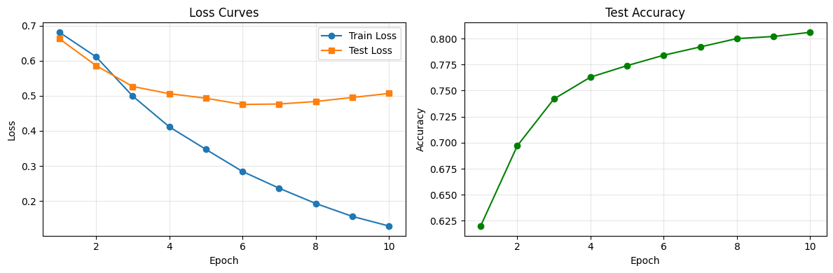
What should we look for?
Both losses decreasing together: Good — the model is learning and generalizing
Train loss dropping while test loss rises: Overfitting! The model is memorizing training data
Neither loss decreasing: The learning rate might be too low, the model too small, or the data too noisy
Loss jumping erratically: The learning rate is probably too high
Regularization: Fighting Overfitting
As neural networks get larger and train longer, they can start memorizing the training data instead of learning general patterns. This is overfitting — training accuracy keeps climbing, but test accuracy plateaus or drops.
The most popular weapon against overfitting in neural networks is dropout. During training, dropout randomly sets a fraction of the neurons’ outputs to zero at each forward pass. This forces the network to spread its learned features across many neurons — no single neuron can become a critical bottleneck.
class FeedForwardWithDropout(nn.Module):
    def __init__(self, vocab_size, embed_dim, hidden_dim, num_classes, dropout=0.5):
        super().__init__()
        self.embedding = nn.Embedding(vocab_size, embed_dim, padding_idx=0)
        self.fc1 = nn.Linear(embed_dim, hidden_dim)
        self.relu = nn.ReLU()
        self.dropout = nn.Dropout(dropout)
        self.fc2 = nn.Linear(hidden_dim, num_classes)

    def forward(self, x):
        embeds = self.embedding(x)
        mask = (x != 0).unsqueeze(-1).float()
        pooled = (embeds * mask).sum(dim=1) / mask.sum(dim=1).clamp(min=1)
        hidden = self.dropout(self.relu(self.fc1(pooled)))
        output = self.fc2(hidden)
        return output

model_dropout = FeedForwardWithDropout(len(vocab), 64, 128, 2, dropout=0.5)
print(model_dropout)
FeedForwardWithDropout(
(embedding): Embedding(10000, 64, padding_idx=0)
(fc1): Linear(in_features=64, out_features=128, bias=True)
(relu): ReLU()
(dropout): Dropout(p=0.5, inplace=False)
(fc2): Linear(in_features=128, out_features=2, bias=True)
)
A critical detail: dropout behaves differently during training and evaluation. During training (model.train()), it randomly zeroes 50% of neurons. During evaluation (model.eval()), dropout is turned off and all neurons contribute — their outputs are scaled so the overall magnitude stays consistent. PyTorch handles this switch automatically.
Another simple technique is early stopping: monitor the test loss during training and stop when it starts increasing. This prevents the model from training past the point of diminishing returns.
Wrap-Up
Key Takeaways
What’s Next
We’ve seen that feed-forward networks can classify text effectively, but they have a major limitation: they throw away word order. Our mean-pooling approach treats “not good” and “good not” identically — clearly a problem for sentiment analysis!
In the next lecture, we’ll explore Recurrent Neural Networks (RNNs) — architectures designed specifically for sequential data. RNNs process text one word at a time while maintaining a “memory” of what came before. We’ll see how this solves the word-order problem, encounter the infamous vanishing gradient issue, and discover how LSTMs provide the fix. This journey from feed-forward to recurrent networks sets the stage for the attention mechanism and Transformers in Week 6.