Lab: Neural Text Classification

CAP-6640: Computational Understanding of Natural Language
Spencer Lyon

Prerequisites

L05.01: Feed-forward networks, PyTorch nn.Module, training loops
L05.02: RNNs, LSTMs, vanishing gradients

Outcomes

Build and train an LSTM-based text classifier in PyTorch from scratch
Reuse and adapt a data pipeline and training loop across different architectures
Compare feed-forward and LSTM classifiers using loss curves, accuracy, and training time
Diagnose training behavior from visualizations and experiment with hyperparameters

References

Lab Overview¶

In Parts 01 and 02 we covered the theory behind feed-forward and recurrent neural networks. Now it’s time to put them to the test.

Here’s our game plan:

Reuse the IMDB data pipeline from Part 01 — vocabulary, encoding, data loaders
Build the feed-forward classifier (from Part 01) and a new LSTM classifier
Train both on the same data with the same hyperparameters
Compare them head-to-head — accuracy, loss curves, training time, and how they handle tricky sentences

The big question: does the LSTM’s ability to process word order actually produce better results? The answer may surprise you.

Setup: Data Pipeline¶

We’ll reuse the exact data pipeline from Part 01. If this code looks familiar, it should — the only new piece is a reusable train_model function that works with any architecture.

import torch
import torch.nn as nn
from torch.utils.data import DataLoader, TensorDataset
from datasets import load_dataset
from collections import Counter
import matplotlib.pyplot as plt
import time

# Load IMDB — same subset and seed as Part 01
dataset = load_dataset("imdb")
train_data = dataset["train"].shuffle(seed=42).select(range(5000))
test_data = dataset["test"].shuffle(seed=42).select(range(1000))

def build_vocab(texts, max_vocab=10000):
    """Build a vocabulary mapping words to integer indices."""
    counter = Counter()
    for text in texts:
        counter.update(text.lower().split())
    vocab = {"<pad>": 0, "<unk>": 1}
    for word, _ in counter.most_common(max_vocab - 2):
        vocab[word] = len(vocab)
    return vocab

def encode_texts(texts, vocab, max_len=256):
    """Convert texts to padded integer sequences."""
    encoded = []
    for text in texts:
        tokens = text.lower().split()[:max_len]
        indices = [vocab.get(t, vocab["<unk>"]) for t in tokens]
        indices += [vocab["<pad>"]] * (max_len - len(indices))
        encoded.append(indices)
    return torch.tensor(encoded)

vocab = build_vocab(train_data["text"])
X_train = encode_texts(train_data["text"], vocab)
y_train = torch.tensor(train_data["label"])
X_test = encode_texts(test_data["text"], vocab)
y_test = torch.tensor(test_data["label"])

train_loader = DataLoader(TensorDataset(X_train, y_train), batch_size=64, shuffle=True)
test_loader = DataLoader(TensorDataset(X_test, y_test), batch_size=64)

print(f"Vocabulary size: {len(vocab):,}")
print(f"Training set:    {X_train.shape}")
print(f"Test set:        {X_test.shape}")

Vocabulary size: 10,000
Training set:    torch.Size([5000, 256])
Test set:        torch.Size([1000, 256])

A Reusable Training Function¶

Instead of writing a training loop twice, let’s write one function that works with any nn.Module. It returns a history dictionary with loss curves, accuracy, training time, and parameter count — everything we need for comparison.

def train_model(model, train_loader, test_loader, epochs=10, lr=0.001):
    """Train a model and return training history with metrics."""
    criterion = nn.CrossEntropyLoss()
    optimizer = torch.optim.Adam(model.parameters(), lr=lr)

    history = {"train_loss": [], "test_loss": [], "test_acc": []}
    start_time = time.time()

    for epoch in range(epochs):
        # Training
        model.train()
        epoch_loss = 0
        for X_batch, y_batch in train_loader:
            optimizer.zero_grad()
            output = model(X_batch)
            loss = criterion(output, y_batch)
            loss.backward()
            optimizer.step()
            epoch_loss += loss.item()
        history["train_loss"].append(epoch_loss / len(train_loader))

        # Evaluation
        model.eval()
        test_loss = 0
        correct = 0
        total = 0
        with torch.no_grad():
            for X_batch, y_batch in test_loader:
                output = model(X_batch)
                test_loss += criterion(output, y_batch).item()
                preds = output.argmax(dim=1)
                correct += (preds == y_batch).sum().item()
                total += len(y_batch)

        history["test_loss"].append(test_loss / len(test_loader))
        history["test_acc"].append(correct / total)

        print(
            f"  Epoch {epoch+1:2d} | "
            f"Train Loss: {history['train_loss'][-1]:.4f} | "
            f"Test Loss: {history['test_loss'][-1]:.4f} | "
            f"Test Acc: {history['test_acc'][-1]:.3f}"
        )

    history["time"] = time.time() - start_time
    history["params"] = sum(p.numel() for p in model.parameters())
    return history

Model 1: Feed-Forward Baseline¶

This is the same FeedForwardClassifier from Part 01: embedding → mean pooling → hidden layer → output. It ignores word order entirely.

class FeedForwardClassifier(nn.Module):
    def __init__(self, vocab_size, embed_dim, hidden_dim, num_classes):
        super().__init__()
        self.embedding = nn.Embedding(vocab_size, embed_dim, padding_idx=0)
        self.fc1 = nn.Linear(embed_dim, hidden_dim)
        self.relu = nn.ReLU()
        self.fc2 = nn.Linear(hidden_dim, num_classes)

    def forward(self, x):
        embeds = self.embedding(x)
        mask = (x != 0).unsqueeze(-1).float()
        pooled = (embeds * mask).sum(dim=1) / mask.sum(dim=1).clamp(min=1)
        hidden = self.relu(self.fc1(pooled))
        return self.fc2(hidden)

torch.manual_seed(42)
ff_model = FeedForwardClassifier(len(vocab), embed_dim=64, hidden_dim=128, num_classes=2)

print("=== Training Feed-Forward Classifier ===\n")
ff_history = train_model(ff_model, train_loader, test_loader)
print(f"\nTraining time: {ff_history['time']:.1f}s | Parameters: {ff_history['params']:,}")

=== Training Feed-Forward Classifier ===

  Epoch  1 | Train Loss: 0.6800 | Test Loss: 0.6661 | Test Acc: 0.611

  Epoch  2 | Train Loss: 0.6127 | Test Loss: 0.5922 | Test Acc: 0.689

  Epoch  3 | Train Loss: 0.5032 | Test Loss: 0.5227 | Test Acc: 0.731

  Epoch  4 | Train Loss: 0.4096 | Test Loss: 0.4828 | Test Acc: 0.767

  Epoch  5 | Train Loss: 0.3349 | Test Loss: 0.4687 | Test Acc: 0.781

  Epoch  6 | Train Loss: 0.2750 | Test Loss: 0.4638 | Test Acc: 0.789

  Epoch  7 | Train Loss: 0.2244 | Test Loss: 0.4654 | Test Acc: 0.799

  Epoch  8 | Train Loss: 0.1922 | Test Loss: 0.4881 | Test Acc: 0.792

  Epoch  9 | Train Loss: 0.1467 | Test Loss: 0.5075 | Test Acc: 0.804

  Epoch 10 | Train Loss: 0.1175 | Test Loss: 0.5077 | Test Acc: 0.809

Training time: 6.3s | Parameters: 648,578

Model 2: LSTM Classifier¶

Now let’s build the LSTM version. The key architectural change: instead of averaging all word embeddings into one vector (which discards word order), we pass the embeddings through an LSTM and use the final hidden state as our document representation.

class LSTMClassifier(nn.Module):
    def __init__(self, vocab_size, embed_dim, hidden_dim, num_classes):
        super().__init__()
        self.embedding = nn.Embedding(vocab_size, embed_dim, padding_idx=0)
        self.lstm = nn.LSTM(embed_dim, hidden_dim, batch_first=True)
        self.fc = nn.Linear(hidden_dim, num_classes)

    def forward(self, x):
        embeds = self.embedding(x)                 # (batch, seq_len, embed_dim)
        output, (h_n, c_n) = self.lstm(embeds)     # h_n: (1, batch, hidden_dim)
        hidden = h_n.squeeze(0)                    # (batch, hidden_dim)
        return self.fc(hidden)                     # (batch, num_classes)

Notice how simple the swap is — we replaced mean pool + linear + relu + linear with LSTM + linear. The LSTM’s hidden state already contains a non-linear, sequence-aware representation, so one output layer is enough.

Let’s trace the shapes to make sure everything connects:

temp_model = LSTMClassifier(len(vocab), embed_dim=64, hidden_dim=128, num_classes=2)
sample = X_train[:2]

with torch.no_grad():
    print(f"Input:           {sample.shape}")
    embeds = temp_model.embedding(sample)
    print(f"After embedding: {embeds.shape}")
    output, (h_n, c_n) = temp_model.lstm(embeds)
    print(f"LSTM outputs:    {output.shape}")
    print(f"Final hidden:    {h_n.shape}")
    hidden = h_n.squeeze(0)
    print(f"Squeezed:        {hidden.shape}")
    logits = temp_model.fc(hidden)
    print(f"Final output:    {logits.shape}")

del temp_model

Input:           torch.Size([2, 256])
After embedding: torch.Size([2, 256, 64])
LSTM outputs:    torch.Size([2, 256, 128])
Final hidden:    torch.Size([1, 2, 128])
Squeezed:        torch.Size([2, 128])
Final output:    torch.Size([2, 2])

Now let’s train it:

torch.manual_seed(42)
lstm_model = LSTMClassifier(len(vocab), embed_dim=64, hidden_dim=128, num_classes=2)

print("=== Training LSTM Classifier ===\n")
lstm_history = train_model(lstm_model, train_loader, test_loader)
print(f"\nTraining time: {lstm_history['time']:.1f}s | Parameters: {lstm_history['params']:,}")

=== Training LSTM Classifier ===

  Epoch  1 | Train Loss: 0.6936 | Test Loss: 0.6960 | Test Acc: 0.494

  Epoch  2 | Train Loss: 0.6861 | Test Loss: 0.7019 | Test Acc: 0.494

  Epoch  3 | Train Loss: 0.6725 | Test Loss: 0.7046 | Test Acc: 0.503

  Epoch  4 | Train Loss: 0.6453 | Test Loss: 0.7238 | Test Acc: 0.499

  Epoch  5 | Train Loss: 0.6043 | Test Loss: 0.7555 | Test Acc: 0.495

  Epoch  6 | Train Loss: 0.5582 | Test Loss: 0.8113 | Test Acc: 0.498

  Epoch  7 | Train Loss: 0.5266 | Test Loss: 0.8899 | Test Acc: 0.505

  Epoch  8 | Train Loss: 0.5004 | Test Loss: 0.9725 | Test Acc: 0.505

  Epoch  9 | Train Loss: 0.4864 | Test Loss: 0.9580 | Test Acc: 0.507

  Epoch 10 | Train Loss: 0.5034 | Test Loss: 0.9906 | Test Acc: 0.511

Training time: 152.9s | Parameters: 739,586

The LSTM takes noticeably longer to train — it must process each of the 256 time steps sequentially, while the feed-forward model processes the entire sequence in one matrix operation. This is exactly the scalability limitation that motivates Transformers (Week 6).

Exercise 5.8: Adding Dropout to the LSTM

Overfitting is a common problem with LSTMs. Add dropout to the LSTMClassifier in two places:

Between the embedding and LSTM — randomly drop some embedding dimensions
Between the LSTM output and the final linear layer — regularize the hidden representation

class LSTMWithDropout(nn.Module):
    def __init__(self, vocab_size, embed_dim, hidden_dim, num_classes, dropout=0.3):
        super().__init__()
        self.embedding = nn.Embedding(vocab_size, embed_dim, padding_idx=0)
        # TODO: add dropout layer(s)
        self.lstm = nn.LSTM(embed_dim, hidden_dim, batch_first=True)
        self.fc = nn.Linear(hidden_dim, num_classes)

    def forward(self, x):
        embeds = self.embedding(x)
        # TODO: apply dropout to embeddings
        output, (h_n, c_n) = self.lstm(embeds)
        hidden = h_n.squeeze(0)
        # TODO: apply dropout to hidden state
        return self.fc(hidden)

Train your LSTMWithDropout with dropout=0.3 and compare its test accuracy and loss curves to the version without dropout. Does regularization help?

Head-to-Head Comparison¶

Let’s see how our two architectures stack up.

Loss Curves and Accuracy¶

epochs = range(1, 11)

fig, axes = plt.subplots(1, 3, figsize=(15, 4))

# Training loss
axes[0].plot(epochs, ff_history["train_loss"], marker="o", label="Feed-Forward")
axes[0].plot(epochs, lstm_history["train_loss"], marker="s", label="LSTM")
axes[0].set_xlabel("Epoch")
axes[0].set_ylabel("Loss")
axes[0].set_title("Training Loss")
axes[0].legend()
axes[0].grid(True, alpha=0.3)

# Test loss
axes[1].plot(epochs, ff_history["test_loss"], marker="o", label="Feed-Forward")
axes[1].plot(epochs, lstm_history["test_loss"], marker="s", label="LSTM")
axes[1].set_xlabel("Epoch")
axes[1].set_ylabel("Loss")
axes[1].set_title("Test Loss")
axes[1].legend()
axes[1].grid(True, alpha=0.3)

# Test accuracy
axes[2].plot(epochs, ff_history["test_acc"], marker="o", label="Feed-Forward")
axes[2].plot(epochs, lstm_history["test_acc"], marker="s", label="LSTM")
axes[2].set_xlabel("Epoch")
axes[2].set_ylabel("Accuracy")
axes[2].set_title("Test Accuracy")
axes[2].legend()
axes[2].grid(True, alpha=0.3)

plt.tight_layout()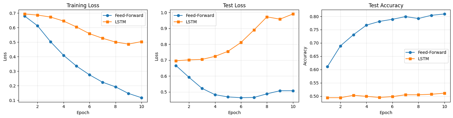

Summary Table¶

print(f"{'Metric':<25} {'Feed-Forward':>15} {'LSTM':>15}")
print("-" * 57)
print(f"{'Parameters':<25} {ff_history['params']:>15,} {lstm_history['params']:>15,}")
print(f"{'Training time':<25} {ff_history['time']:>14.1f}s {lstm_history['time']:>14.1f}s")
print(f"{'Best test accuracy':<25} {max(ff_history['test_acc']):>15.3f} {max(lstm_history['test_acc']):>15.3f}")
print(f"{'Final test accuracy':<25} {ff_history['test_acc'][-1]:>15.3f} {lstm_history['test_acc'][-1]:>15.3f}")
print(f"{'Final train loss':<25} {ff_history['train_loss'][-1]:>15.4f} {lstm_history['train_loss'][-1]:>15.4f}")
print(f"{'Final test loss':<25} {ff_history['test_loss'][-1]:>15.4f} {lstm_history['test_loss'][-1]:>15.4f}")

Metric                       Feed-Forward            LSTM
---------------------------------------------------------
Parameters                        648,578         739,586
Training time                        6.3s          152.9s
Best test accuracy                  0.809           0.511
Final test accuracy                 0.809           0.511
Final train loss                   0.1175          0.5034
Final test loss                    0.5077          0.9906

What Do We See?¶

A few observations worth discussing:

Training time: The LSTM is significantly slower. Processing 256 tokens sequentially is inherently more expensive than averaging them in one operation. This gap grows with sequence length — and it’s the core motivation behind Transformers.
Accuracy: On this particular task (sentiment analysis on relatively short reviews), the performance gap between the two architectures may be modest. Sentiment is often carried by a few key words (“great”, “terrible”, “boring”) regardless of their position, which plays to the feed-forward model’s strengths.
Parameters: The LSTM has more parameters due to its gate matrices ( $4 \times$ the parameters of an equivalently-sized feed-forward hidden layer).
Overfitting: Check the gap between training and test loss. Which model overfits more?

The lesson here is important: a more complex model isn’t automatically better. The LSTM’s ability to model word order is a genuine advantage, but whether it matters depends on the task and data.

Testing on Tricky Sentences¶

Let’s see how both models handle sentences where word order really matters:

def predict_review(model, text, vocab):
    """Predict sentiment for a single review."""
    model.eval()
    encoded = encode_texts([text], vocab)
    with torch.no_grad():
        output = model(encoded)
        probs = torch.softmax(output, dim=1)
        pred = output.argmax(dim=1).item()
    label = "positive" if pred == 1 else "negative"
    confidence = probs[0, pred].item()
    return label, confidence

test_sentences = [
    "This movie was absolutely brilliant and moving",
    "This movie was terrible and boring",
    "This movie was not good",
    "Not my favorite, but I would watch it again",
    "Despite great acting, the plot was weak and unconvincing",
]

print(f"{'Sentence':<55} {'FF Pred':>10} {'FF Conf':>8} {'LSTM Pred':>10} {'LSTM Conf':>8}")
print("-" * 95)

for sent in test_sentences:
    ff_label, ff_conf = predict_review(ff_model, sent, vocab)
    lstm_label, lstm_conf = predict_review(lstm_model, sent, vocab)
    short = sent[:52] + "..." if len(sent) > 55 else sent
    print(f"{short:<55} {ff_label:>10} {ff_conf:>8.3f} {lstm_label:>10} {lstm_conf:>8.3f}")

Sentence                                                   FF Pred  FF Conf  LSTM Pred LSTM Conf
-----------------------------------------------------------------------------------------------
This movie was absolutely brilliant and moving            positive    0.998   negative    0.500
This movie was terrible and boring                        negative    1.000   negative    0.500
This movie was not good                                   negative    0.972   negative    0.500
Not my favorite, but I would watch it again               positive    0.997   negative    0.500
Despite great acting, the plot was weak and unconvin...   negative    1.000   negative    0.500

Pay attention to the sentences with negation (“not good”) and contrast (“despite great acting... weak”). These are the cases where word order matters most, and where we’d expect the LSTM to have an advantage.

Exercise 5.9: Error Analysis

Pick 10 reviews from the test set where the two models disagree on the prediction, and analyze the results.

# Find reviews where the models disagree
ff_model.eval()
lstm_model.eval()

disagreements = []
with torch.no_grad():
    ff_preds = ff_model(X_test).argmax(dim=1)
    lstm_preds = lstm_model(X_test).argmax(dim=1)

    for i in range(len(X_test)):
        if ff_preds[i] != lstm_preds[i]:
            disagreements.append(i)

print(f"Models disagree on {len(disagreements)} out of {len(X_test)} test reviews")

# Examine the first 10 disagreements
for idx in disagreements[:10]:
    text = test_data[idx]["text"][:150]
    true_label = "pos" if y_test[idx] == 1 else "neg"
    ff_label = "pos" if ff_preds[idx] == 1 else "neg"
    lstm_label = "pos" if lstm_preds[idx] == 1 else "neg"
    # TODO: print and analyze each disagreement

(a) For each disagreement, which model got the correct answer?

(b) Do the disagreements share any patterns? (e.g., negation, sarcasm, long sentences, mixed sentiment)

(c) Overall, does the LSTM win more disagreements than the feed-forward? What does this tell you?

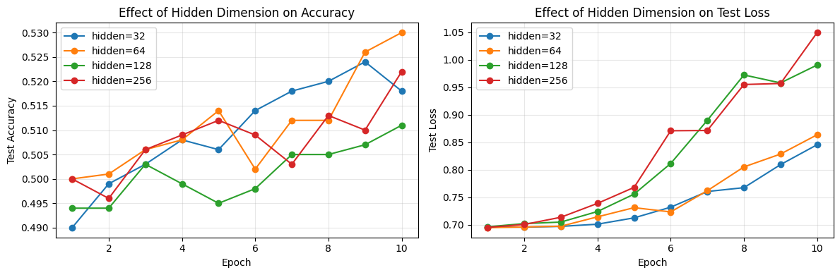
Hyperparameter Experiments¶

Which hyperparameters matter most for neural text classifiers? Let’s run a quick experiment varying the hidden dimension size for the LSTM. We’ll keep everything else fixed (embed_dim=64, lr=0.001, 10 epochs) and compare hidden sizes of 32, 64, 128, and 256.

hidden_dims = [32, 64, 128, 256]
results = {}

for hd in hidden_dims:
    print(f"\n--- Hidden dim = {hd} ---")
    torch.manual_seed(42)
    model = LSTMClassifier(len(vocab), embed_dim=64, hidden_dim=hd, num_classes=2)
    history = train_model(model, train_loader, test_loader, epochs=10)
    results[hd] = history

# Plot comparison
fig, (ax1, ax2) = plt.subplots(1, 2, figsize=(12, 4))

for hd in hidden_dims:
    ax1.plot(range(1, 11), results[hd]["test_acc"], marker="o", label=f"hidden={hd}")
    ax2.plot(range(1, 11), results[hd]["test_loss"], marker="o", label=f"hidden={hd}")

ax1.set_xlabel("Epoch")
ax1.set_ylabel("Test Accuracy")
ax1.set_title("Effect of Hidden Dimension on Accuracy")
ax1.legend()
ax1.grid(True, alpha=0.3)

ax2.set_xlabel("Epoch")
ax2.set_ylabel("Test Loss")
ax2.set_title("Effect of Hidden Dimension on Test Loss")
ax2.legend()
ax2.grid(True, alpha=0.3)

plt.tight_layout()


--- Hidden dim = 32 ---

  Epoch  1 | Train Loss: 0.6943 | Test Loss: 0.6959 | Test Acc: 0.490

  Epoch  2 | Train Loss: 0.6884 | Test Loss: 0.6953 | Test Acc: 0.499

  Epoch  3 | Train Loss: 0.6819 | Test Loss: 0.6968 | Test Acc: 0.503

  Epoch  4 | Train Loss: 0.6702 | Test Loss: 0.7008 | Test Acc: 0.508

  Epoch  5 | Train Loss: 0.6480 | Test Loss: 0.7123 | Test Acc: 0.506

  Epoch  6 | Train Loss: 0.6197 | Test Loss: 0.7318 | Test Acc: 0.514

  Epoch  7 | Train Loss: 0.5865 | Test Loss: 0.7603 | Test Acc: 0.518

  Epoch  8 | Train Loss: 0.5524 | Test Loss: 0.7673 | Test Acc: 0.520

  Epoch  9 | Train Loss: 0.5299 | Test Loss: 0.8093 | Test Acc: 0.524

  Epoch 10 | Train Loss: 0.5154 | Test Loss: 0.8455 | Test Acc: 0.518

--- Hidden dim = 64 ---

  Epoch  1 | Train Loss: 0.6946 | Test Loss: 0.6944 | Test Acc: 0.500

  Epoch  2 | Train Loss: 0.6869 | Test Loss: 0.6957 | Test Acc: 0.501

  Epoch  3 | Train Loss: 0.6752 | Test Loss: 0.6971 | Test Acc: 0.506

  Epoch  4 | Train Loss: 0.6526 | Test Loss: 0.7142 | Test Acc: 0.508

  Epoch  5 | Train Loss: 0.6222 | Test Loss: 0.7309 | Test Acc: 0.514

  Epoch  6 | Train Loss: 0.6339 | Test Loss: 0.7231 | Test Acc: 0.502

  Epoch  7 | Train Loss: 0.5623 | Test Loss: 0.7618 | Test Acc: 0.512

  Epoch  8 | Train Loss: 0.5304 | Test Loss: 0.8050 | Test Acc: 0.512

  Epoch  9 | Train Loss: 0.5094 | Test Loss: 0.8285 | Test Acc: 0.526

  Epoch 10 | Train Loss: 0.4904 | Test Loss: 0.8636 | Test Acc: 0.530

--- Hidden dim = 128 ---

  Epoch  1 | Train Loss: 0.6936 | Test Loss: 0.6960 | Test Acc: 0.494

  Epoch  2 | Train Loss: 0.6861 | Test Loss: 0.7019 | Test Acc: 0.494

  Epoch  3 | Train Loss: 0.6725 | Test Loss: 0.7046 | Test Acc: 0.503

  Epoch  4 | Train Loss: 0.6453 | Test Loss: 0.7238 | Test Acc: 0.499

  Epoch  5 | Train Loss: 0.6043 | Test Loss: 0.7555 | Test Acc: 0.495

  Epoch  6 | Train Loss: 0.5582 | Test Loss: 0.8113 | Test Acc: 0.498

  Epoch  7 | Train Loss: 0.5266 | Test Loss: 0.8899 | Test Acc: 0.505

  Epoch  8 | Train Loss: 0.5004 | Test Loss: 0.9725 | Test Acc: 0.505

  Epoch  9 | Train Loss: 0.4864 | Test Loss: 0.9580 | Test Acc: 0.507

  Epoch 10 | Train Loss: 0.5034 | Test Loss: 0.9906 | Test Acc: 0.511

--- Hidden dim = 256 ---

  Epoch  1 | Train Loss: 0.6943 | Test Loss: 0.6949 | Test Acc: 0.500

  Epoch  2 | Train Loss: 0.6835 | Test Loss: 0.7002 | Test Acc: 0.496

  Epoch  3 | Train Loss: 0.6642 | Test Loss: 0.7134 | Test Acc: 0.506

  Epoch  4 | Train Loss: 0.6310 | Test Loss: 0.7387 | Test Acc: 0.509

  Epoch  5 | Train Loss: 0.5887 | Test Loss: 0.7678 | Test Acc: 0.512

  Epoch  6 | Train Loss: 0.5366 | Test Loss: 0.8709 | Test Acc: 0.509

  Epoch  7 | Train Loss: 0.5103 | Test Loss: 0.8714 | Test Acc: 0.503

  Epoch  8 | Train Loss: 0.4988 | Test Loss: 0.9551 | Test Acc: 0.513

  Epoch  9 | Train Loss: 0.4852 | Test Loss: 0.9570 | Test Acc: 0.510

  Epoch 10 | Train Loss: 0.4813 | Test Loss: 1.0496 | Test Acc: 0.522

print(f"\n{'Hidden Dim':<12} {'Params':>10} {'Time':>8} {'Best Acc':>10} {'Final Acc':>10}")
print("-" * 54)
for hd in hidden_dims:
    r = results[hd]
    print(f"{hd:<12} {r['params']:>10,} {r['time']:>7.1f}s {max(r['test_acc']):>10.3f} {r['test_acc'][-1]:>10.3f}")


Hidden Dim       Params     Time   Best Acc  Final Acc
------------------------------------------------------
32              652,610    45.5s      0.524      0.518
64              673,410    86.4s      0.530      0.530
128             739,586   194.3s      0.511      0.511
256             970,242   489.0s      0.522      0.522

Notice the trade-off: larger hidden dimensions give the model more capacity but also more parameters and longer training time. At some point you hit diminishing returns — or even overfitting, where a bigger model memorizes training data without generalizing better.

Exercise 5.10: Embedding Dimension Experiment

Run a similar experiment, but this time vary the embedding dimension instead of the hidden dimension. Test embed_dim values of 16, 32, 64, and 128, keeping hidden_dim=128 fixed.

embed_dims = [16, 32, 64, 128]
embed_results = {}

for ed in embed_dims:
    torch.manual_seed(42)
    model = LSTMClassifier(len(vocab), embed_dim=ed, hidden_dim=128, num_classes=2)
    history = train_model(model, train_loader, test_loader, epochs=10)
    embed_results[ed] = history
    # TODO: plot and compare results

(a) Which embedding dimension gives the best test accuracy?

(b) How does embedding dimension affect the total parameter count? Why?

(c) Based on your results from this exercise and the hidden dimension experiment above, which hyperparameter has a bigger impact on performance: embedding size or hidden size?

Wrap-Up¶

Key Takeaways¶

Key Takeaways

A reusable training function makes it easy to compare architectures — same data, same hyperparameters, same evaluation, different model
The LSTM classifier replaces mean pooling with sequential processing: embedding → LSTM → final hidden state → linear output — and the code change is surprisingly small
LSTMs are significantly slower to train than feed-forward networks due to their sequential nature — this is the fundamental scalability problem that Transformers solve
More complex isn’t always better: on tasks where a few key words dominate (like sentiment), feed-forward models can be competitive with LSTMs despite ignoring word order
Loss curves and accuracy plots reveal training dynamics at a glance — watch for diverging train/test curves as a sign of overfitting
Hyperparameters matter: hidden dimension and embedding dimension both affect capacity, but there are diminishing returns — finding the sweet spot requires experimentation

What’s Next¶

We’ve now explored the full arc from classical machine learning (Week 4) through feed-forward networks to LSTMs. Along the way, we’ve seen a recurring trade-off: more powerful architectures capture more structure but cost more to train.

In Week 6, we’ll meet the architecture that changed everything: the Transformer. By replacing recurrence with self-attention, Transformers process all tokens in parallel while maintaining the ability to capture long-range dependencies. We’ll build the attention mechanism from scratch and see exactly how it solves the limitations we encountered this week.