Recurrent Networks and the Road to Attention

CAP-6640: Computational Understanding of Natural Language
Spencer Lyon

Prerequisites

L05.01: Feed-forward networks, PyTorch basics (nn.Module, training loops, backpropagation)
L03.02: Word embeddings and dense representations

Outcomes

Explain why sequential data requires architectures with memory and how RNNs address this
Trace the flow of information through an RNN, identifying how hidden states capture temporal dependencies
Diagnose the vanishing gradient problem and explain how LSTM gates solve it
Describe the encoder-decoder (seq2seq) architecture for variable-length sequence tasks
Identify the bottleneck problem in seq2seq models and explain how attention provides a solution

References

Why Order Matters¶

In Part 01 we built a feed-forward sentiment classifier that worked by averaging word embeddings. It achieved reasonable accuracy, but let’s think about what it can’t do.

Consider these two sentences:

“The movie was not good” — negative
“The movie was good, not great” — positive (mildly)

Our mean-pooling classifier sees the same bag of words in both cases — “not” and “good” are both present. It has no way to distinguish “not good” from “good not” because it throws away word order entirely. For a sentiment classifier, that’s a serious blind spot.

The problem is fundamental: feed-forward networks process a fixed-size input and produce a fixed-size output. They have no concept of sequence or position. But language is inherently sequential — the meaning of a word often depends on what came before it.

What we need is a network with memory — one that processes words one at a time, building up an understanding of the sentence as it goes. That’s exactly what Recurrent Neural Networks provide.

Recurrent Neural Networks: Adding Memory¶

The Core Idea¶

A Recurrent Neural Network processes a sequence one element at a time, maintaining a hidden state $h_t$ that serves as a running summary of everything it has seen so far. At each time step $t$ , the RNN takes two inputs:

The current word’s embedding $x_t$
The previous hidden state $h_{t-1}$

And produces a new hidden state:

h_t = \tanh(W_{xh} \, x_t + W_{hh} \, h_{t-1} + b_h)

(1)

That’s the entire RNN in one equation. The weight matrix $W_{xh}$ determines how the current input influences the new hidden state. The matrix $W_{hh}$ determines how the previous hidden state carries forward. The tanh squashes everything into the range $(-1, 1)$ .

The crucial insight: the same weights are reused at every time step. The RNN doesn’t learn separate parameters for position 1, position 2, etc. — it learns a single transformation that it applies repeatedly. This is what makes it able to handle sequences of any length.

Processing a Sequence Step by Step¶

Let’s trace an RNN processing a sentence word by word. We’ll use small dimensions so you can see the actual numbers:

import torch
import torch.nn as nn
import numpy as np
import matplotlib.pyplot as plt

# Small dimensions so we can see what's happening
embed_dim = 4
hidden_dim = 3

torch.manual_seed(42)
rnn_cell = nn.RNNCell(input_size=embed_dim, hidden_size=hidden_dim)

# Imagine these are embeddings for "the movie was great"
words = ["the", "movie", "was", "great"]
embeddings = torch.randn(len(words), embed_dim)

# Start with a zero hidden state
h = torch.zeros(1, hidden_dim)
print(f"h₀ = {[f'{v:.2f}' for v in h.squeeze().tolist()]}")
print()

for i, word in enumerate(words):
    x = embeddings[i].unsqueeze(0)  # (1, embed_dim)
    h = rnn_cell(x, h)
    print(f"After '{word:>5s}':  h = {[f'{v:.2f}' for v in h.squeeze().tolist()]}")

print(f"\nThe final hidden state encodes the entire sentence.")

h₀ = ['0.00', '0.00', '0.00']

After '  the':  h = ['-0.98', '-0.90', '0.54']
After 'movie':  h = ['-0.92', '-0.63', '0.22']
After '  was':  h = ['-0.96', '-0.74', '0.13']
After 'great':  h = ['-0.97', '-0.91', '0.92']

The final hidden state encodes the entire sentence.

Notice how the hidden state changes at every step. After “the”, it captures something about the article. After “the movie”, it’s been updated to reflect both words. By the end, the final hidden state $h_4$ is a compressed representation of the entire sentence “the movie was great.”

The Full RNN in PyTorch¶

In practice, we don’t loop manually — PyTorch’s nn.RNN processes entire sequences efficiently:

# Full RNN: processes all time steps at once (internally still sequential)
rnn = nn.RNN(input_size=64, hidden_size=128, batch_first=True)

# Batch of 2 sequences, each 10 tokens long, each token a 64-d embedding
x = torch.randn(2, 10, 64)

output, h_n = rnn(x)

print(f"Input shape:              {x.shape}")      # (batch, seq_len, embed)
print(f"All hidden states shape:  {output.shape}")  # (batch, seq_len, hidden)
print(f"Final hidden state shape: {h_n.shape}")     # (layers, batch, hidden)

Input shape:              torch.Size([2, 10, 64])
All hidden states shape:  torch.Size([2, 10, 128])
Final hidden state shape: torch.Size([1, 2, 128])

Two outputs here:

output: the hidden state at every time step — useful when we need per-token predictions (like NER)
h_n: the hidden state at the last time step — useful for sequence classification (one label for the whole document)

For classification, we’d take h_n and feed it through a linear layer to get class scores — exactly like the feed-forward architecture from Part 01, but using a sequence-aware representation instead of a naive average.

# Verify: the last output IS the final hidden state
print(f"Last output matches h_n: {torch.allclose(output[0, -1], h_n[0, 0])}")

Last output matches h_n: True

The Vanishing Gradient Problem¶

RNNs sound great in theory, but in practice they have a devastating weakness. Consider a long movie review:

“The director, who previously won an award for his groundbreaking documentary about climate change in Southeast Asia, has once again demonstrated remarkable skill in this latest production, which I found to be absolutely brilliant.”

To classify this as positive, the network needs to connect “brilliant” all the way back to “The director.” That means during backpropagation, the gradient signal must flow backward through every single time step.

Here’s the problem: at each step, the gradient gets multiplied by the recurrent weight matrix $W_{hh}$ . If the effective multiplier is less than 1, the gradient shrinks exponentially:

# Why gradients vanish: repeated multiplication through time
print("Gradient magnitude after N steps of backpropagation:")
print(f"{'Steps':>6} | {'Scale':>14} | {'% Remaining':>12}")
print("-" * 38)
for n in [1, 5, 10, 20, 50, 100]:
    scale = 0.9 ** n
    print(f"{n:6d} | {scale:14.8f} | {scale*100:11.4f}%")

Gradient magnitude after N steps of backpropagation:
 Steps |          Scale |  % Remaining
--------------------------------------
     1 |     0.90000000 |     90.0000%
     5 |     0.59049000 |     59.0490%
    10 |     0.34867844 |     34.8678%
    20 |     0.12157665 |     12.1577%
    50 |     0.00515378 |      0.5154%
   100 |     0.00002656 |      0.0027%

After just 50 steps, a gradient that started at 1.0 has shrunk to less than 1% of its original value. After 100 steps, it’s effectively zero. The network can’t learn from signals that don’t survive the journey.

steps = np.arange(1, 101)

fig, axes = plt.subplots(1, 2, figsize=(12, 4))

for factor in [0.5, 0.7, 0.9, 0.99]:
    axes[0].plot(steps, factor ** steps, label=f"factor = {factor}")
axes[0].set_xlabel("Steps Back in Time")
axes[0].set_ylabel("Gradient Scale")
axes[0].set_title("Vanishing Gradients (factor < 1)")
axes[0].legend()
axes[0].grid(True, alpha=0.3)

for factor in [1.01, 1.1, 1.5, 2.0]:
    values = np.minimum(factor ** steps, 1e15)
    axes[1].plot(steps, values, label=f"factor = {factor}")
axes[1].set_xlabel("Steps Back in Time")
axes[1].set_ylabel("Gradient Scale (log)")
axes[1].set_title("Exploding Gradients (factor > 1)")
axes[1].set_yscale("log")
axes[1].legend()
axes[1].grid(True, alpha=0.3)

plt.tight_layout()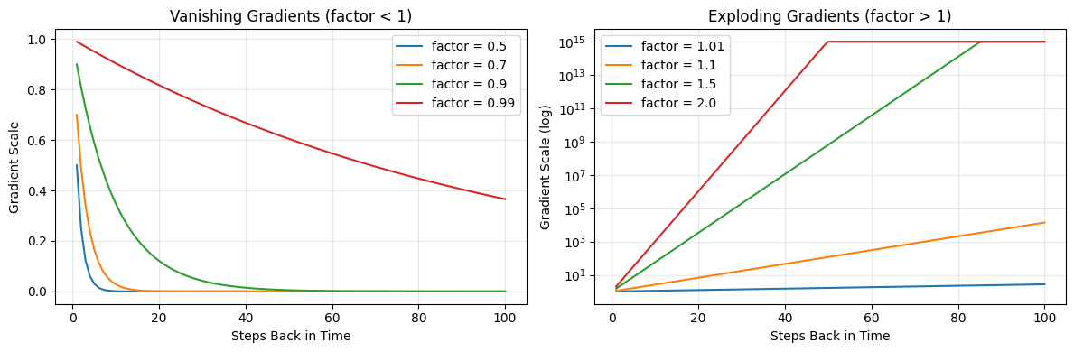

The left plot shows vanishing gradients — the signal dies out, and the model can’t learn long-range dependencies. The right plot shows the opposite problem: exploding gradients, where the signal grows uncontrollably. Exploding gradients are easier to fix (just clip the gradient to a maximum norm), but vanishing gradients require a fundamentally different architecture.

This is the problem that motivated the most important advance in recurrent networks: the LSTM.

LSTM: Gated Memory¶

The Key Insight¶

The core problem with vanilla RNNs is that information has no choice but to pass through the same transformation at every step — getting squashed by tanh each time. What if we gave the network an explicit, separate memory channel that information can flow through more easily?

That’s exactly what a Long Short-Term Memory network does. An LSTM maintains two vectors at each time step:

Hidden state $h_t$ : the “working memory,” similar to a vanilla RNN
Cell state $c_t$ : the “long-term memory,” a highway where information can flow across many time steps with minimal transformation

The cell state is the breakthrough. Instead of passing through tanh at every step, information in the cell state is regulated by gates — learned switches that decide what to remember, what to forget, and what to output.

The Four Components¶

An LSTM cell has four learned components:

1. Forget gate — What should we erase from long-term memory?

f_t = \sigma(W_f [h_{t-1}, x_t] + b_f)

(2)

The sigmoid outputs values between 0 and 1 for each dimension of the cell state. A value near 0 means “forget this,” near 1 means “keep this.” When the model reads “not” after storing positive sentiment, the forget gate can learn to erase that positive signal.

2. Input gate — What new information should we store?

i_t = \sigma(W_i [h_{t-1}, x_t] + b_i)

(3)

3. Candidate values — What are the proposed new values?

\tilde{c}_t = \tanh(W_c [h_{t-1}, x_t] + b_c)

(4)

4. Cell state update — Combine forgetting with new information:

c_t = f_t \odot c_{t-1} + i_t \odot \tilde{c}_t

(5)

This is the critical equation. The $\odot$ symbol means element-wise multiplication. The cell state is updated by selectively forgetting old information ( $f_t \odot c_{t-1}$ ) and selectively adding new information ( $i_t \odot \tilde{c}_t$ ). Because this is an addition (not a multiplication through tanh), gradients can flow through the cell state across many time steps without vanishing.

5. Output gate — What part of the cell state do we reveal?

o_t = \sigma(W_o [h_{t-1}, x_t] + b_o)

(6)

h_t = o_t \odot \tanh(c_t)

(7)

The hidden state $h_t$ is a filtered view of the cell state — the LSTM decides what information is relevant for the current output.

LSTM in PyTorch¶

Using an LSTM in PyTorch is almost identical to using an RNN — the key difference is that you get back both the hidden state and the cell state:

lstm = nn.LSTM(input_size=64, hidden_size=128, batch_first=True)

x = torch.randn(2, 10, 64)  # Same input shape as our RNN example

output, (h_n, c_n) = lstm(x)

print(f"Input shape:              {x.shape}")
print(f"All hidden states shape:  {output.shape}")    # (2, 10, 128)
print(f"Final hidden state shape: {h_n.shape}")       # (1, 2, 128)
print(f"Final cell state shape:   {c_n.shape}")       # (1, 2, 128)
print()
print("Key difference from nn.RNN: LSTM returns BOTH h_n AND c_n")
print("The cell state c_n is the long-term memory that flows through the gates")

Input shape:              torch.Size([2, 10, 64])
All hidden states shape:  torch.Size([2, 10, 128])
Final hidden state shape: torch.Size([1, 2, 128])
Final cell state shape:   torch.Size([1, 2, 128])

Key difference from nn.RNN: LSTM returns BOTH h_n AND c_n
The cell state c_n is the long-term memory that flows through the gates

GRU: A Simplified Alternative¶

The Gated Recurrent Unit is a popular simplification of the LSTM that combines the forget and input gates into a single “update gate” and merges the cell state and hidden state. It has fewer parameters and is often faster to train, while achieving comparable performance on many tasks. PyTorch provides it as nn.GRU with the same interface as nn.RNN.

Beyond Classification: Sequence-to-Sequence Models¶

So far we’ve used RNNs and LSTMs for classification — mapping a variable-length sequence to a single label. But many NLP tasks require mapping one sequence to another sequence:

Machine translation: “The cat sat on the mat” → “Le chat s’est assis sur le tapis”
Summarization: a long article → a short summary
Question answering: (question, context) → answer text

The input and output can have completely different lengths. A 5-word English sentence might become a 7-word French sentence. How do we handle this?

The Encoder-Decoder Architecture¶

The sequence-to-sequence (seq2seq) model solves this with a two-part design:

Encoder: An LSTM that reads the entire input sequence and compresses it into a fixed-size context vector — the final hidden state
Decoder: A separate LSTM that takes the context vector as its initial state and generates the output sequence, one token at a time

The encoder and decoder are separate networks with their own learned weights. The only connection between them is the context vector — the encoder’s final hidden state becomes the decoder’s initial hidden state.

Let’s see this in PyTorch:

# === Encoder ===
encoder = nn.LSTM(input_size=64, hidden_size=128, batch_first=True)

# Source: "The cat sat" — 3 tokens, each a 64-d embedding
source = torch.randn(1, 3, 64)
enc_outputs, (enc_h, enc_c) = encoder(source)

print("=== Encoder ===")
print(f"Source sequence:   {source.shape}")       # (1, 3, 64)
print(f"Encoder outputs:   {enc_outputs.shape}")  # (1, 3, 128)
print(f"Context vector h:  {enc_h.shape}")        # (1, 1, 128)
print(f"Context vector c:  {enc_c.shape}")        # (1, 1, 128)

=== Encoder ===
Source sequence:   torch.Size([1, 3, 64])
Encoder outputs:   torch.Size([1, 3, 128])
Context vector h:  torch.Size([1, 1, 128])
Context vector c:  torch.Size([1, 1, 128])

# === Decoder ===
decoder = nn.LSTM(input_size=64, hidden_size=128, batch_first=True)

# Target: "Le chat assis <EOS>" — 4 tokens (different length from source!)
target = torch.randn(1, 4, 64)

# Initialize decoder with encoder's final state
dec_outputs, (dec_h, dec_c) = decoder(target, (enc_h, enc_c))

print("=== Decoder ===")
print(f"Target sequence:   {target.shape}")       # (1, 4, 64)
print(f"Decoder outputs:   {dec_outputs.shape}")  # (1, 4, 128)
print()
print("The decoder produces one output per target token.")
print("Each output would be projected to the vocabulary to predict the next word.")

=== Decoder ===
Target sequence:   torch.Size([1, 4, 64])
Decoder outputs:   torch.Size([1, 4, 128])

The decoder produces one output per target token.
Each output would be projected to the vocabulary to predict the next word.

At each time step, the decoder produces a hidden state that is projected through a linear layer to vocabulary-size logits, then through softmax to get a probability distribution over all possible next words. The highest-probability word is selected and fed back as input to the next decoder step. This auto-regressive process continues until the model generates a special end-of-sequence token.

The Bottleneck Problem¶

Look at the shape of our context vector: (1, 1, 128). That’s a single 128-dimensional vector that must encode everything about the source sentence — every word, every relationship, every nuance.

For a 3-word sentence, that might be fine. But what about a 50-word paragraph? A 500-word document? We’re asking a fixed-size vector to carry an unbounded amount of information. This is the information bottleneck.

# The bottleneck: same size context regardless of input length
for src_len in [5, 20, 50, 200]:
    source = torch.randn(1, src_len, 64)
    _, (h, c) = encoder(source)
    print(f"Source length: {src_len:>3d} tokens → Context vector: {h.shape} (always 128-d!)")

Source length:   5 tokens → Context vector: torch.Size([1, 1, 128]) (always 128-d!)
Source length:  20 tokens → Context vector: torch.Size([1, 1, 128]) (always 128-d!)
Source length:  50 tokens → Context vector: torch.Size([1, 1, 128]) (always 128-d!)
Source length: 200 tokens → Context vector: torch.Size([1, 1, 128]) (always 128-d!)

The bottleneck has a predictable consequence: seq2seq models perform well on short sequences but degrade significantly on longer ones. The decoder simply doesn’t have enough information to reconstruct the details of a long source sequence from a single vector.

What if, instead of compressing everything into one vector, the decoder could look back at the encoder’s hidden states at every position? That’s the key insight behind the attention mechanism.

The Origins of Attention¶

The attention mechanism, introduced by Bahdanau et al. (2014), addresses the bottleneck problem with an elegant idea: instead of forcing all source information through a single context vector, let the decoder attend to all encoder hidden states at each generation step.

Here’s the intuition. When translating “The cat sat on the mat” to French and generating the word “chat” (cat), the decoder doesn’t need information about “mat” — it needs to focus on “cat.” At the next step, when generating “assis” (sat), it should focus on “sat.” Attention makes this dynamic focus possible.

At each decoder step $t$ , attention works in three stages:

Score: Compute how relevant each encoder state $h_i^{enc}$ is to the current decoder state $h_t^{dec}$
Normalize: Convert scores to weights using softmax (so they sum to 1)
Combine: Take a weighted sum of encoder states to get a context vector specific to this decoder step

\alpha_{t,i} = \frac{\exp(\text{score}(h_t^{dec}, h_i^{enc}))}{\sum_j \exp(\text{score}(h_t^{dec}, h_j^{enc}))} \qquad c_t = \sum_i \alpha_{t,i} \, h_i^{enc}

(8)

The key difference from vanilla seq2seq: instead of one context vector for the entire sequence, we get a different context vector at each decoder step — one that focuses on the most relevant parts of the source.

This was a transformative idea, and it directly paved the way to the Transformer architecture (Week 6). In fact, the “Attention Is All You Need” paper that introduced Transformers asked: if attention is the most important part of the model, why keep the recurrent part at all? Their answer — self-attention without any recurrence — delivered two massive advantages:

Parallelization: RNNs must process tokens sequentially (token 5 depends on token 4 which depends on token 3...). Attention can process all tokens simultaneously, making it dramatically faster on modern GPUs.
Direct long-range connections: In an RNN, information from token 1 must pass through every intermediate hidden state to reach token 50. With attention, token 50 can directly attend to token 1 — no information loss from the journey.

These advantages are why Transformers replaced RNNs as the dominant architecture for NLP. We’ll explore exactly how in Week 6.

Wrap-Up¶

Key Takeaways¶

Key Takeaways

RNNs process sequences one token at a time, maintaining a hidden state $h_t$ that encodes everything seen so far — this gives them a sense of word order that feed-forward networks lack
The vanishing gradient problem makes it nearly impossible for vanilla RNNs to learn long-range dependencies — gradients shrink exponentially as they backpropagate through time
LSTMs solve this with a separate cell state and learned gates (forget, input, output) that control what information to keep, add, or reveal — the additive cell update lets gradients flow across many time steps
Sequence-to-sequence models use an encoder-decoder architecture to map variable-length inputs to variable-length outputs, enabling tasks like translation and summarization
The information bottleneck in seq2seq models — compressing all source information into a single fixed-size vector — degrades performance on longer sequences
Attention solves the bottleneck by letting the decoder look at all encoder states at each step, creating a dynamic, step-specific context vector that focuses on the most relevant source information
Transformers take attention to its logical conclusion: remove recurrence entirely, gaining parallelization and direct long-range connections — setting the stage for modern LLMs

What’s Next¶

In the lab (Part 03), we’ll put theory into practice by implementing both a feed-forward and an LSTM-based text classifier in PyTorch, training them on the same dataset, and comparing their performance head-to-head. You’ll experiment with hyperparameters — embedding size, hidden dimensions, dropout — and visualize training dynamics to build real intuition for how these architectures behave. With the conceptual foundation from Parts 01 and 02, you’ll be well-prepared to understand why one architecture outperforms the other on different types of text.