Lab: Attention from Scratch

CAP-6640: Computational Understanding of Natural Language
Spencer Lyon

Prerequisites

L06.01: The Transformer architecture — Q/K/V, scaled dot-product attention, multi-head attention, masking, residual connections, layer normalization, positional encoding
PyTorch basics: nn.Module, nn.Linear, tensor operations, @ for matrix multiplication

Outcomes

Implement scaled dot-product attention from scratch in PyTorch and verify correctness against the built-in implementation
Build a multi-head attention module that properly splits, computes, and recombines attention across heads
Assemble a complete transformer block by combining attention, residual connections, layer normalization, and a feed-forward network
Visualize and interpret real attention patterns from a pretrained BERT model
Experiment with positional encoding to observe its effect on attention behavior

References

J&M Chapter 8: Transformers
HF Transformers Documentation
Karpathy’s nanoGPT — a clean, minimal GPT implementation
D2L Chapter 11: Attention Mechanisms and Transformers

Overview¶

In L06.01, we studied the Transformer architecture from the top down — understanding what each component does and why it’s there. Now it’s time to build it from the bottom up.

In this lab, you will:

Implement scaled dot-product attention from the formula
Build a multi-head attention module (inspired by nanoGPT)
Assemble a complete transformer block
Visualize attention patterns from a real pretrained model
Experiment with positional encodings and their effects

By the end, you’ll have built every core component of the Transformer with your own hands — and you’ll be able to see what these components learn on real text.

Setup¶

import torch
import torch.nn as nn
import torch.nn.functional as F
import math
import matplotlib.pyplot as plt
import numpy as np

torch.manual_seed(42)
print(f"PyTorch version: {torch.__version__}")

PyTorch version: 2.10.0+cu128

Exercise 6.5: Scaled Dot-Product Attention¶

Let’s start with the most fundamental operation in the Transformer. Recall from L06.01 the formula for scaled dot-product attention:

\text{Attention}(Q, K, V) = \text{softmax}\left(\frac{QK^T}{\sqrt{d_k}}\right)V

(1)

Your task is to implement this as a Python function. The function should:

Compute the dot product $QK^T$
Scale by $\sqrt{d_k}$ (the last dimension of $Q$ )
Optionally apply a mask (setting masked positions to $-\infty$ before softmax)
Apply softmax to get attention weights
Multiply weights by $V$ to get the output

Exercise 6.5: Implement Scaled Dot-Product Attention

Complete the function below. It should handle both masked and unmasked attention.

Hint: Use scores.masked_fill(mask == 0, float('-inf')) to apply the mask. The mask is a tensor of 1s (attend) and 0s (ignore).

def scaled_dot_product_attention(Q, K, V, mask=None):
    """
    Compute scaled dot-product attention.

    Args:
        Q: Queries  (..., seq_len, d_k)
        K: Keys     (..., seq_len, d_k)
        V: Values   (..., seq_len, d_v)
        mask: Optional mask tensor of 1s and 0s (..., seq_len, seq_len)

    Returns:
        output: Weighted combination of values (..., seq_len, d_v)
        weights: Attention weights (..., seq_len, seq_len)
    """
    d_k = Q.size(-1)

    # Step 1: Compute raw attention scores
    # TODO

    # Step 2: Scale by sqrt(d_k)
    # TODO

    # Step 3: Apply mask (if provided)
    # TODO

    # Step 4: Softmax to get attention weights
    # TODO

    # Step 5: Weighted combination of values
    # TODO

    return output, weights

Testing Your Implementation¶

Once you’ve implemented the function, run the cell below to verify it works correctly. We’ll compare your output against PyTorch’s built-in F.scaled_dot_product_attention.

# Test data
torch.manual_seed(42)
seq_len, d_k = 6, 16
Q = torch.randn(seq_len, d_k)
K = torch.randn(seq_len, d_k)
V = torch.randn(seq_len, d_k)

# --- Uncomment after implementing scaled_dot_product_attention ---
# # Test without mask
# output, weights = scaled_dot_product_attention(Q, K, V)
# print(f"Output shape:  {output.shape}  (expected: [{seq_len}, {d_k}])")
# print(f"Weights shape: {weights.shape}  (expected: [{seq_len}, {seq_len}])")
# print(f"Weights row sums: {weights.sum(dim=-1).round(decimals=2).tolist()}  (should all be 1.0)")
#
# # Verify against PyTorch built-in
# ref = F.scaled_dot_product_attention(Q.unsqueeze(0), K.unsqueeze(0), V.unsqueeze(0)).squeeze(0)
# max_diff = (output - ref).abs().max().item()
# print(f"\nMax difference vs PyTorch built-in: {max_diff:.2e}")
# assert max_diff < 1e-6, f"Difference too large: {max_diff}"
# print("✓ Matches PyTorch's implementation!")

# Test with causal mask
# --- Uncomment after implementing scaled_dot_product_attention ---
# causal_mask = torch.tril(torch.ones(seq_len, seq_len))
# output_masked, weights_masked = scaled_dot_product_attention(Q, K, V, mask=causal_mask)
#
# # Check that future positions get zero weight
# upper_triangle_weight = (weights_masked * (1 - causal_mask)).sum().item()
# print(f"Weight on masked (future) positions: {upper_triangle_weight:.8f}  (should be ~0)")
# assert upper_triangle_weight < 1e-6, "Masked positions should have zero weight!"
# print("✓ Causal masking works correctly!")

Exercise 6.6: Multi-Head Attention¶

A single attention head learns one “perspective” on token relationships. Multi-head attention runs $h$ heads in parallel, each attending to different aspects of the input, then combines the results.

The clean pattern from nanoGPT uses a single linear projection to compute Q, K, V for all heads at once, then reshapes to separate the heads. Here’s the shape flow:

Input x:            (batch, seq_len, d_model)
    ↓ c_attn (single linear: d_model → 3 * d_model)
Q, K, V:            (batch, seq_len, d_model)  — each
    ↓ reshape + transpose
Q, K, V per head:   (batch, n_heads, seq_len, d_k)  — where d_k = d_model / n_heads
    ↓ attention per head
Output per head:    (batch, n_heads, seq_len, d_k)
    ↓ transpose + reshape (concatenate heads)
Concatenated:       (batch, seq_len, d_model)
    ↓ c_proj (linear: d_model → d_model)
Final output:       (batch, seq_len, d_model)

Exercise 6.6: Implement Multi-Head Attention

Complete the MultiHeadAttention class below. Use the scaled_dot_product_attention function you built in Exercise 6.5.

Key operations you’ll need:

tensor.view(B, T, n_heads, d_k) to reshape
.transpose(1, 2) to move the head dimension before the sequence dimension
.contiguous().view(B, T, C) to recombine heads

class MultiHeadAttention(nn.Module):
    def __init__(self, d_model, n_heads):
        super().__init__()
        assert d_model % n_heads == 0, "d_model must be divisible by n_heads"
        self.n_heads = n_heads
        self.d_k = d_model // n_heads

        # Single linear layer for all Q, K, V projections (nanoGPT pattern)
        self.c_attn = nn.Linear(d_model, 3 * d_model)
        # Output projection
        self.c_proj = nn.Linear(d_model, d_model)

    def forward(self, x, mask=None):
        B, T, C = x.size()  # batch, sequence length, d_model

        # Step 1: Project to Q, K, V and split
        # TODO: use self.c_attn, then split into q, k, v

        # Step 2: Reshape for multi-head: (B, T, C) -> (B, n_heads, T, d_k)
        # TODO: view + transpose for q, k, v

        # Step 3: Compute attention (use your function from Ex 6.5)
        # TODO

        # Step 4: Recombine heads: (B, n_heads, T, d_k) -> (B, T, C)
        # TODO: transpose + contiguous + view

        # Step 5: Output projection
        # TODO

        return output, weights

Testing Multi-Head Attention¶

# --- Uncomment after implementing MultiHeadAttention ---
# torch.manual_seed(42)
# d_model, n_heads = 64, 4
# mha = MultiHeadAttention(d_model, n_heads)
#
# x = torch.randn(2, 8, d_model)  # batch=2, seq_len=8
# output, weights = mha(x)
#
# print(f"Input shape:   {x.shape}")
# print(f"Output shape:  {output.shape}   (should match input)")
# print(f"Weights shape: {weights.shape}  (batch, n_heads, seq_len, seq_len)")
#
# assert output.shape == x.shape, f"Shape mismatch: {output.shape} != {x.shape}"
# assert weights.shape == (2, n_heads, 8, 8), f"Weight shape wrong: {weights.shape}"
# print("✓ Multi-head attention shapes are correct!")
#
# # Count parameters
# n_params = sum(p.numel() for p in mha.parameters())
# print(f"\nParameters: {n_params:,}")
# print(f"  c_attn (Q,K,V): {d_model} × {3*d_model} + {3*d_model} bias = {d_model*3*d_model + 3*d_model:,}")
# print(f"  c_proj (output): {d_model} × {d_model} + {d_model} bias = {d_model*d_model + d_model:,}")

Exercise 6.7: The Transformer Block¶

With attention and a feed-forward network in hand, we can assemble a complete transformer block. Recall from L06.01 that the block follows this pattern (using pre-norm, the modern default):

\begin{align} x &= x + \text{MultiHeadAttention}(\text{LayerNorm}(x)) \\ x &= x + \text{FeedForward}(\text{LayerNorm}(x)) \end{align}

(2)

Each sublayer has a residual connection (the + x) and layer normalization applied before the sublayer. This is the exact pattern used in nanoGPT’s Block class:

# From nanoGPT model.py — just 4 lines!
def forward(self, x):
    x = x + self.attn(self.ln_1(x))
    x = x + self.mlp(self.ln_2(x))
    return x

Exercise 6.7: Build a Transformer Block

Complete the TransformerBlock class below. You’ll need your MultiHeadAttention from Exercise 6.6 and the FeedForward class provided.

class FeedForward(nn.Module):
    """Position-wise feed-forward network with 4x expansion."""
    def __init__(self, d_model):
        super().__init__()
        self.net = nn.Sequential(
            nn.Linear(d_model, 4 * d_model),
            nn.GELU(),
            nn.Linear(4 * d_model, d_model),
        )

    def forward(self, x):
        return self.net(x)


class TransformerBlock(nn.Module):
    def __init__(self, d_model, n_heads):
        super().__init__()
        self.ln1 = nn.LayerNorm(d_model)
        self.attn = MultiHeadAttention(d_model, n_heads)
        self.ln2 = nn.LayerNorm(d_model)
        self.ffn = FeedForward(d_model)

    def forward(self, x, mask=None):
        # TODO: Apply pre-norm self-attention with residual connection
        # TODO: Apply pre-norm feed-forward with residual connection
        return x, weights

Testing the Transformer Block¶

# --- Uncomment after implementing TransformerBlock ---
# torch.manual_seed(42)
# d_model, n_heads = 64, 4
# block = TransformerBlock(d_model, n_heads)
#
# x = torch.randn(2, 8, d_model)
# output, weights = block(x)
#
# print(f"Input shape:  {x.shape}")
# print(f"Output shape: {output.shape}")
# assert output.shape == x.shape, "Transformer block should preserve input shape!"
# print("✓ Shape preserved through transformer block!")
#
# # Verify the residual connection works: output should be different from input
# # but not wildly different (the residual keeps it close)
# diff = (output - x).abs().mean().item()
# print(f"\nMean absolute change from residual: {diff:.4f}")
# print("  (Small but nonzero means residual connections + sublayers are working)")
#
# # Count parameters
# n_params = sum(p.numel() for p in block.parameters())
# print(f"\nTotal parameters in block: {n_params:,}")

Stacking Blocks¶

A complete Transformer is just a stack of identical blocks. Let’s see how parameters scale:

# --- Uncomment after implementing TransformerBlock ---
# # Stack N transformer blocks — like a real model
# d_model, n_heads, n_layers = 64, 4, 6
#
# blocks = nn.ModuleList([TransformerBlock(d_model, n_heads) for _ in range(n_layers)])
# total_params = sum(p.numel() for p in blocks.parameters())
#
# print(f"Architecture: {n_layers} blocks × ({d_model}-dim, {n_heads} heads)")
# print(f"Parameters per block: {sum(p.numel() for p in blocks[0].parameters()):,}")
# print(f"Total parameters:     {total_params:,}")

# For reference, real models:
print("Real model sizes (d_model, n_heads, n_layers, ~params):")
print("  GPT-2 Small:  (768,  12, 12,  ~124M)")
print("  GPT-2 Medium: (1024, 16, 24,  ~350M)")
print("  GPT-2 Large:  (1280, 20, 36,  ~774M)")
print("  GPT-2 XL:     (1600, 25, 48, ~1558M)")

Real model sizes (d_model, n_heads, n_layers, ~params):
  GPT-2 Small:  (768,  12, 12,  ~124M)
  GPT-2 Medium: (1024, 16, 24,  ~350M)
  GPT-2 Large:  (1280, 20, 36,  ~774M)
  GPT-2 XL:     (1600, 25, 48, ~1558M)

Visualizing Real Attention Patterns¶

We’ve built the components — now let’s see what they actually learn. We’ll load a pretrained BERT model and visualize its attention weights on real sentences.

Why BERT? It’s an encoder-only transformer that has been trained on massive amounts of text. Its attention heads have learned meaningful linguistic patterns that we can interpret.

from transformers import AutoTokenizer, AutoModel

# Load pretrained BERT
tokenizer = AutoTokenizer.from_pretrained("bert-base-uncased")
model = AutoModel.from_pretrained("bert-base-uncased", output_attentions=True)
model.eval()

print(f"Model: bert-base-uncased")
print(f"  Layers: 12, Heads: 12, d_model: 768")
print(f"  Total parameters: {sum(p.numel() for p in model.parameters()):,}")

Warning: You are sending unauthenticated requests to the HF Hub. Please set a HF_TOKEN to enable higher rate limits and faster downloads.

BertModel LOAD REPORT from: bert-base-uncased
Key                                        | Status     |  | 
-------------------------------------------+------------+--+-
cls.predictions.bias                       | UNEXPECTED |  | 
cls.predictions.transform.dense.bias       | UNEXPECTED |  | 
cls.predictions.transform.dense.weight     | UNEXPECTED |  | 
cls.predictions.transform.LayerNorm.bias   | UNEXPECTED |  | 
cls.seq_relationship.bias                  | UNEXPECTED |  | 
cls.seq_relationship.weight                | UNEXPECTED |  | 
cls.predictions.transform.LayerNorm.weight | UNEXPECTED |  | 

Notes:
- UNEXPECTED	:can be ignored when loading from different task/architecture; not ok if you expect identical arch.

Model: bert-base-uncased
  Layers: 12, Heads: 12, d_model: 768
  Total parameters: 109,482,240

def get_attention(text, tokenizer, model):
    """Get attention weights for a text from a pretrained model."""
    inputs = tokenizer(text, return_tensors="pt")
    tokens = tokenizer.convert_ids_to_tokens(inputs["input_ids"][0])
    with torch.no_grad():
        outputs = model(**inputs)
    # outputs.attentions: tuple of (batch, n_heads, seq_len, seq_len) per layer
    attentions = torch.stack(outputs.attentions)  # (n_layers, batch, n_heads, seq, seq)
    return tokens, attentions.squeeze(1)  # remove batch dim


def plot_attention_head(tokens, weights, layer, head, ax=None):
    """Plot attention weights for a single head as a heatmap."""
    if ax is None:
        fig, ax = plt.subplots(figsize=(8, 6))

    w = weights[layer, head].numpy()
    im = ax.imshow(w, cmap="Blues", vmin=0, vmax=w.max())
    ax.set_xticks(range(len(tokens)))
    ax.set_yticks(range(len(tokens)))
    ax.set_xticklabels(tokens, rotation=45, ha="right", fontsize=8)
    ax.set_yticklabels(tokens, fontsize=8)
    ax.set_xlabel("Key (attending to)")
    ax.set_ylabel("Query (attending from)")
    ax.set_title(f"Layer {layer}, Head {head}")
    return im

# Let's look at BERT's attention on a sentence with a clear coreference
text = "The cat sat on the mat because it was tired."
tokens, attentions = get_attention(text, tokenizer, model)

print(f"Tokens: {tokens}")
print(f"Attention shape: {attentions.shape}  (layers, heads, seq, seq)")

# Plot a few interesting heads
fig, axes = plt.subplots(1, 3, figsize=(18, 5))

# These layers/heads often show interesting patterns in BERT
for ax, (layer, head) in zip(axes, [(0, 0), (3, 10), (8, 5)]):
    plot_attention_head(tokens, attentions, layer, head, ax=ax)

plt.suptitle(f'BERT attention on: "{text}"', fontsize=12, y=1.02)
plt.tight_layout()
plt.show()

Tokens: ['[CLS]', 'the', 'cat', 'sat', 'on', 'the', 'mat', 'because', 'it', 'was', 'tired', '.', '[SEP]']
Attention shape: torch.Size([12, 12, 13, 13])  (layers, heads, seq, seq)

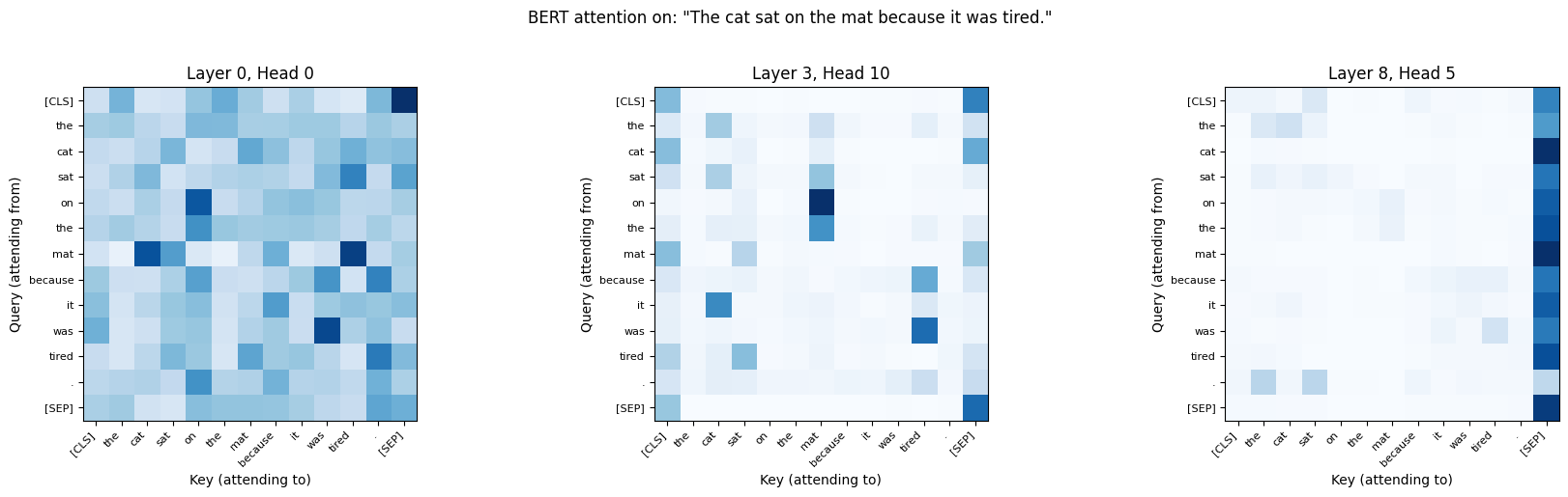
Different heads learn different attention patterns. Research has found that BERT’s heads can specialize:

Positional heads: Attend to adjacent tokens (common in early layers)
Syntactic heads: Track dependency relations (subject-verb, modifier-noun)
Separator heads: Attend to [CLS] or [SEP] tokens (aggregation)
Coreference heads: Link pronouns to their referents

Let’s look for some of these patterns:

# Average attention across all heads in a given layer
text = "The lawyer asked the witness if she remembered the accident."
tokens, attentions = get_attention(text, tokenizer, model)

fig, axes = plt.subplots(1, 3, figsize=(18, 5))
for ax, layer in zip(axes, [0, 5, 11]):
    # Average across all 12 heads
    avg_weights = attentions[layer].mean(dim=0).numpy()
    im = ax.imshow(avg_weights, cmap="Blues", vmin=0)
    ax.set_xticks(range(len(tokens)))
    ax.set_yticks(range(len(tokens)))
    ax.set_xticklabels(tokens, rotation=45, ha="right", fontsize=8)
    ax.set_yticklabels(tokens, fontsize=8)
    ax.set_title(f"Layer {layer} (averaged over 12 heads)")

plt.suptitle("Attention evolves across layers", fontsize=12, y=1.02)
plt.tight_layout()
plt.show()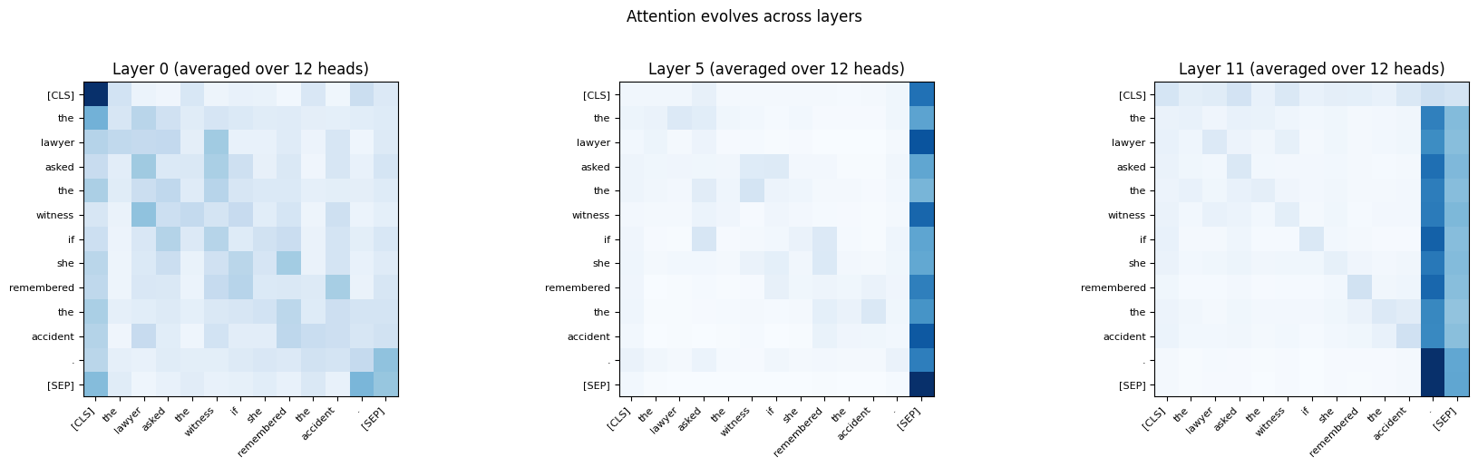

Exercise 6.8: Interpreting Attention Patterns¶

Exercise 6.8: Interpret Attention Patterns

Use the get_attention and plot_attention_head functions above to explore attention patterns on the following sentences. For each, find at least one interesting head and describe what pattern it appears to capture.

Sentence 1 (coreference): "The nurse examined the patient and told him the results."

Sentence 2 (long-range dependency): "The keys that I left on the table are missing."

Sentence 3 (your choice): Pick a sentence with an interesting linguistic phenomenon (ambiguity, negation, etc.)

For each sentence:

Run get_attention to extract attention weights
Explore different layer/head combinations with plot_attention_head
Write 2-3 sentences describing what the head appears to attend to

Tip: Early layers (0-3) often show positional/local patterns. Middle layers (4-8) tend to capture syntactic relationships. Later layers (9-11) often show more abstract or task-specific patterns.

# Example:
text = "The nurse examined the patient and told him the results."
tokens, attentions = get_attention(text, tokenizer, model)

# Explore: try different (layer, head) combinations
fig, ax = plt.subplots(figsize=(8, 6))
plot_attention_head(tokens, attentions, layer=5, head=10, ax=ax)
plt.tight_layout()
plt.show()

Exercise 6.9: Positional Encoding Experiments¶

In L06.01, we learned that positional encoding is essential because self-attention treats its input as an unordered set. But how much does it actually matter? Let’s find out experimentally.

We’ll create a simple setup: take an embedding matrix, add (or don’t add) positional encoding, compute self-attention, and compare the results.

def sinusoidal_positional_encoding(max_len, d_model):
    """Compute sinusoidal positional encoding (from L06.01)."""
    PE = torch.zeros(max_len, d_model)
    position = torch.arange(0, max_len, dtype=torch.float).unsqueeze(1)
    div_term = torch.exp(torch.arange(0, d_model, 2).float() * (-math.log(10000.0) / d_model))
    PE[:, 0::2] = torch.sin(position * div_term)
    PE[:, 1::2] = torch.cos(position * div_term)
    return PE

# Setup: create a sequence with repeated tokens
# If two tokens have the SAME embedding, only positional encoding distinguishes them
torch.manual_seed(42)

d_model = 32
vocab = {"the": 0, "cat": 1, "sat": 2, "on": 3, "mat": 4}
embedding = nn.Embedding(len(vocab), d_model)

# "the cat sat on the mat" — note "the" appears at positions 0 and 4
token_ids = torch.tensor([0, 1, 2, 3, 0, 4])  # the cat sat on the mat
tokens = ["the", "cat", "sat", "on", "the", "mat"]

X = embedding(token_ids)  # (6, 32)
PE = sinusoidal_positional_encoding(6, d_model)

# Compute attention WITHOUT positional encoding
scores_no_pe = (X @ X.transpose(0, 1)) / math.sqrt(d_model)
weights_no_pe = F.softmax(scores_no_pe, dim=-1)

# Compute attention WITH positional encoding
X_pe = X + PE
scores_with_pe = (X_pe @ X_pe.transpose(0, 1)) / math.sqrt(d_model)
weights_with_pe = F.softmax(scores_with_pe, dim=-1)

# Compare
fig, axes = plt.subplots(1, 2, figsize=(14, 5))

for ax, w, title in zip(axes,
                         [weights_no_pe, weights_with_pe],
                         ["WITHOUT Positional Encoding", "WITH Positional Encoding"]):
    im = ax.imshow(w.detach().numpy(), cmap="Blues", vmin=0)
    ax.set_xticks(range(len(tokens)))
    ax.set_yticks(range(len(tokens)))
    ax.set_xticklabels(tokens, rotation=45, ha="right")
    ax.set_yticklabels(tokens)
    ax.set_title(title)
    plt.colorbar(im, ax=ax)

plt.suptitle('Effect of positional encoding on "the cat sat on the mat"', y=1.02)
plt.tight_layout()
plt.show()

# Highlight the key difference
print("Attention weights FROM 'the' (pos 0) and 'the' (pos 4):")
print(f"  Without PE — row 0: {weights_no_pe[0].detach().round(decimals=3).tolist()}")
print(f"  Without PE — row 4: {weights_no_pe[4].detach().round(decimals=3).tolist()}")
print(f"  With PE    — row 0: {weights_with_pe[0].detach().round(decimals=3).tolist()}")
print(f"  With PE    — row 4: {weights_with_pe[4].detach().round(decimals=3).tolist()}")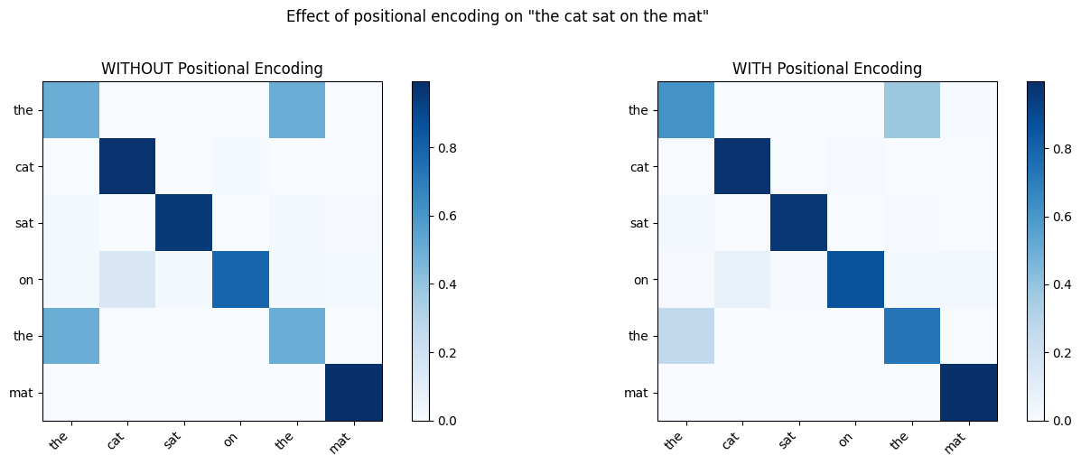

Attention weights FROM 'the' (pos 0) and 'the' (pos 4):
  Without PE — row 0: [0.49799999594688416, 0.0, 0.0020000000949949026, 0.0, 0.49799999594688416, 0.0010000000474974513]
  Without PE — row 4: [0.49799999594688416, 0.0, 0.0020000000949949026, 0.0, 0.49799999594688416, 0.0010000000474974513]
  With PE    — row 0: [0.6169999837875366, 0.0010000000474974513, 0.0020000000949949026, 0.0, 0.375, 0.004999999888241291]
  With PE    — row 4: [0.26100000739097595, 0.0, 0.0010000000474974513, 0.0010000000474974513, 0.734000027179718, 0.003000000026077032]

Wrap-Up¶

Key Takeaways¶

Key Takeaways

Scaled dot-product attention can be implemented in ~5 lines of PyTorch: compute $QK^T$ , scale, optionally mask, softmax, then multiply by $V$
Multi-head attention uses a single linear projection for all Q/K/V, then reshapes to split across heads — no extra cost compared to one large head
The transformer block is remarkably simple: LayerNorm → Attention → Residual → LayerNorm → FFN → Residual — just 2 lines in nanoGPT’s Block.forward()
Real attention heads specialize: early layers learn positional patterns, middle layers capture syntax, and later layers develop more abstract representations
Positional encoding is critical for distinguishing identical tokens at different positions — without it, attention treats the input as an unordered bag of embeddings
Verifying against reference implementations (like F.scaled_dot_product_attention or nn.MultiheadAttention) is essential for catching subtle bugs in custom implementations

What’s Next¶

In Week 7, we’ll move from building Transformers to using them. You’ll meet the three major model families — encoder-only (BERT), decoder-only (GPT), and encoder-decoder (T5) — and learn how the Hugging Face ecosystem makes it easy to load, fine-tune, and deploy these pretrained models for real NLP tasks. The components you built today are exactly what’s running inside those models — just scaled up by a factor of 1000x.