The Transformer Architecture

CAP-6640: Computational Understanding of Natural Language
Spencer Lyon

Prerequisites

L05.01: Feed-forward networks, PyTorch basics (nn.Module, nn.Linear, activation functions)
L05.02: RNNs, the seq2seq bottleneck problem, and the intuition behind attention
L03.02: Word embeddings and dense representations

Outcomes

Explain the intuition behind attention as a learned weighted average and describe the roles of queries, keys, and values
Derive and compute scaled dot-product attention from the mathematical formula, including the purpose of the scaling factor
Describe how multi-head attention enables a model to attend to information from different representation subspaces simultaneously
Identify and explain each component of the transformer block: self-attention, residual connections, layer normalization, and feed-forward layers
Explain why positional encoding is necessary for transformers and describe both sinusoidal and learned approaches

References

“Attention Is All You Need”¶

In 2017, a team of researchers at Google published a paper with a bold title: “Attention Is All You Need.” It proposed an architecture called the Transformer that abandoned recurrence entirely — no RNNs, no LSTMs, no sequential processing at all. Instead, it relied on a single mechanism: attention.

The result? A model that was not only faster to train (because it could process all tokens in parallel) but also achieved state-of-the-art results on machine translation. Within a few years, Transformers became the foundation for virtually every major advance in NLP: BERT, GPT, T5, and every LLM you’ve interacted with.

This lecture walks through the Transformer architecture from the ground up. We’ll start with the attention mechanism — the heart of the model — and then examine each supporting component that makes the full architecture work. By the end, you’ll understand every box in the now-famous architecture diagram.

Building Block Review¶

Before we dive into the Transformer, let’s remind ourselves of three fundamental operations that appear throughout the architecture. We covered these in Week 5, but they’ll be everywhere today.

Linear Layers¶

A linear layer (also called a dense or fully-connected layer) is just a matrix multiplication with a bias term:

y = xW + b

(1)

In PyTorch, this is nn.Linear. It transforms an input vector from one dimension to another. The weights $W$ and bias $b$ are learnable parameters — the network adjusts them during training.

Softmax¶

The softmax function takes a vector of arbitrary real numbers and turns it into a probability distribution — all values between 0 and 1, summing to 1:

\text{softmax}(x_i) = \frac{\exp(x_i)}{\sum_j \exp(x_j)}

(2)

Why is this useful? It lets us interpret raw scores (like attention scores) as weights that sum to 1. Larger inputs get exponentially more probability mass.

Normalization¶

Normalization transforms a vector to have mean 0 and variance 1:

\text{norm}(x_i) = \frac{x_i - \mu}{\sigma}

(3)

where $\mu = \frac{1}{N}\sum_i x_i$ and $\sigma^2 = \text{var}(x)$ . This keeps values in a manageable range and stabilizes training. We’ll see a specific form called layer normalization later in this lecture.

import torch
import torch.nn as nn
import torch.nn.functional as F
import matplotlib.pyplot as plt

# Quick demo of these building blocks
x = torch.tensor([2.0, 1.0, 0.5, -1.0, 3.0])

# Softmax: turns scores into a probability distribution
probs = F.softmax(x, dim=-1)
print(f"Input:   {x.tolist()}")
print(f"Softmax: {probs.tolist()}")
print(f"Sum:     {probs.sum().item():.1f}")

Input:   [2.0, 1.0, 0.5, -1.0, 3.0]
Softmax: [0.22940629720687866, 0.08439385890960693, 0.051187463104724884, 0.011421467177569866, 0.6235909461975098]
Sum:     1.0

From RNNs to Attention¶

At the end of Week 5, we identified a fundamental problem with sequence-to-sequence models: the information bottleneck. The encoder compresses an entire input sequence into a single fixed-size vector, and the decoder must reconstruct everything from that one vector. No matter how long the input, the context vector is always the same size.

We also saw the solution: attention. Instead of forcing all information through one vector, attention lets the decoder look back at every encoder hidden state, dynamically deciding which parts of the input are most relevant at each step.

The key question the Transformer paper asked was: if attention is the most powerful part of the model, why keep the recurrent part at all?

Their answer was revolutionary: throw away recurrence entirely. Use attention — and only attention — to capture relationships between all positions in a sequence. This gives us two massive advantages:

Parallelization — RNNs must process tokens sequentially. Attention can process all tokens simultaneously, making it dramatically faster on GPUs.
Direct long-range connections — In an RNN, information from token 1 must pass through every intermediate state to reach token 50. With attention, any token can directly attend to any other token — no information loss from the journey.

The Attention Mechanism¶

So what exactly is attention? At its core, attention is a mechanism that allows a network to selectively focus on different parts of its input depending on context. It quite literally answers the question: “What should I pay attention to when processing this token?”

The mechanism works by taking weighted averages. For each token in a sequence, we compute a set of weights over all other tokens — how relevant is each one? — and then combine the information from all tokens using those weights. Tokens that are more relevant get higher weights.

The key insight is that these weights are not fixed — they are computed from the data itself. The model learns how to determine what’s relevant. This is what makes attention so powerful: it’s a fully differentiable, context-dependent routing of information.

An Intuitive Example¶

Consider the sentence: “The cat sat on the mat because it was tired.”

When processing the word “it,” we need to figure out what “it” refers to. A good attention mechanism would assign high weight to “cat” and low weight to “mat” — because “cat” is the entity that can be “tired.” The model learns to make this connection from data.

Encoder-Decoder Architecture¶

Before we look at attention in detail, let’s understand the high-level framework. The original Transformer uses an encoder-decoder architecture — the same general pattern as seq2seq, but without any recurrence.

The encoder takes an input sequence (e.g., an English sentence) and maps it to a sequence of continuous representations (vectors)
The decoder takes those representations and generates an output sequence (e.g., the French translation), one token at a time

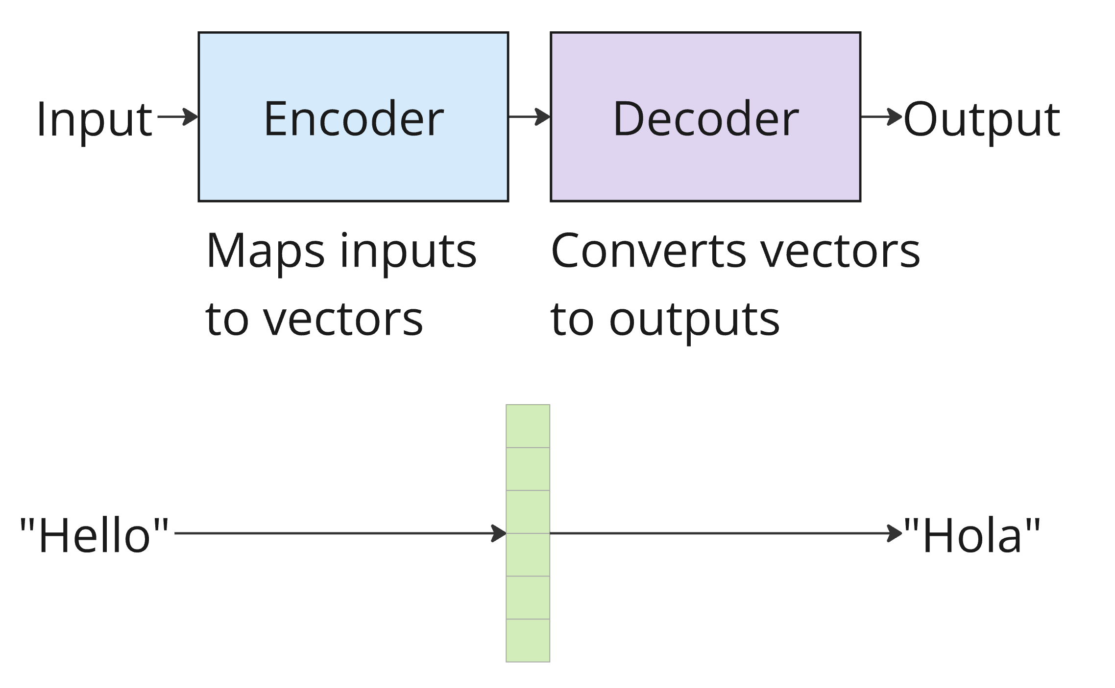
This encoder-decoder structure is natural for tasks where the input and output are different sequences (like translation). Later, we’ll see that many modern models use only the encoder (like BERT) or only the decoder (like GPT), depending on the task.

The Full Transformer Architecture¶

Here is the famous diagram from the original paper. Don’t worry about understanding every piece right now — we’ll walk through each component one by one. But it’s helpful to see the big picture first.

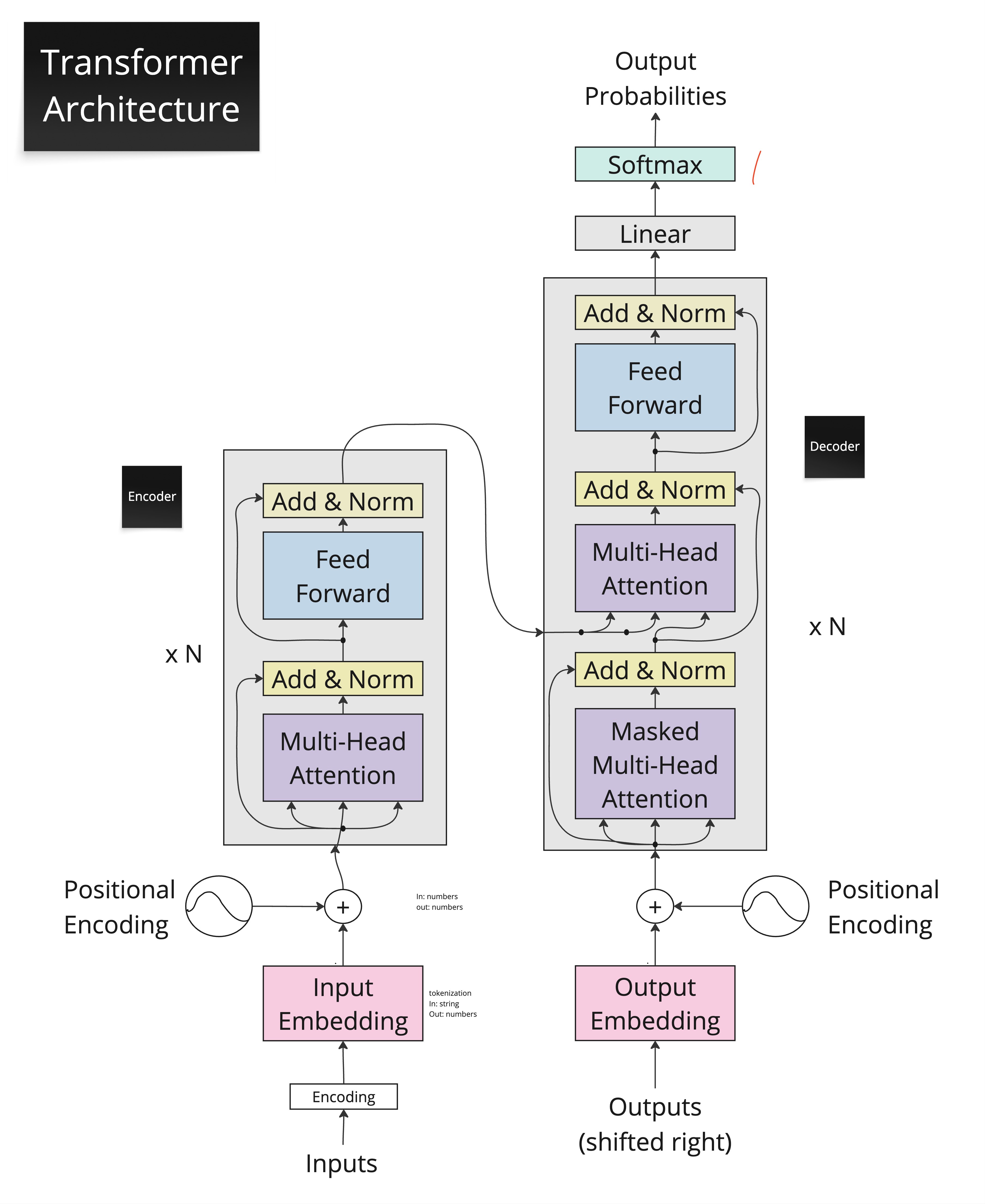
At a glance, here’s what we see:

Encoder side (left):

Input Embedding + Positional Encoding
A stack of N identical blocks, each containing:
- Multi-Head Attention
- Add & Normalize
- Feed-Forward Network
- Add & Normalize

Decoder side (right):

Output Embedding + Positional Encoding
A stack of N identical blocks, each containing:
- Masked Multi-Head Attention
- Add & Normalize
- Multi-Head Attention (cross-attention to encoder output)
- Add & Normalize
- Feed-Forward Network
- Add & Normalize
A final Linear layer + Softmax for output probabilities

The encoder and decoder connect through cross-attention: the decoder’s attention mechanism attends to the encoder’s output representations. This is how the decoder “looks at” the input when generating each output token.

Now let’s examine each component in detail, starting with the heart of the model.

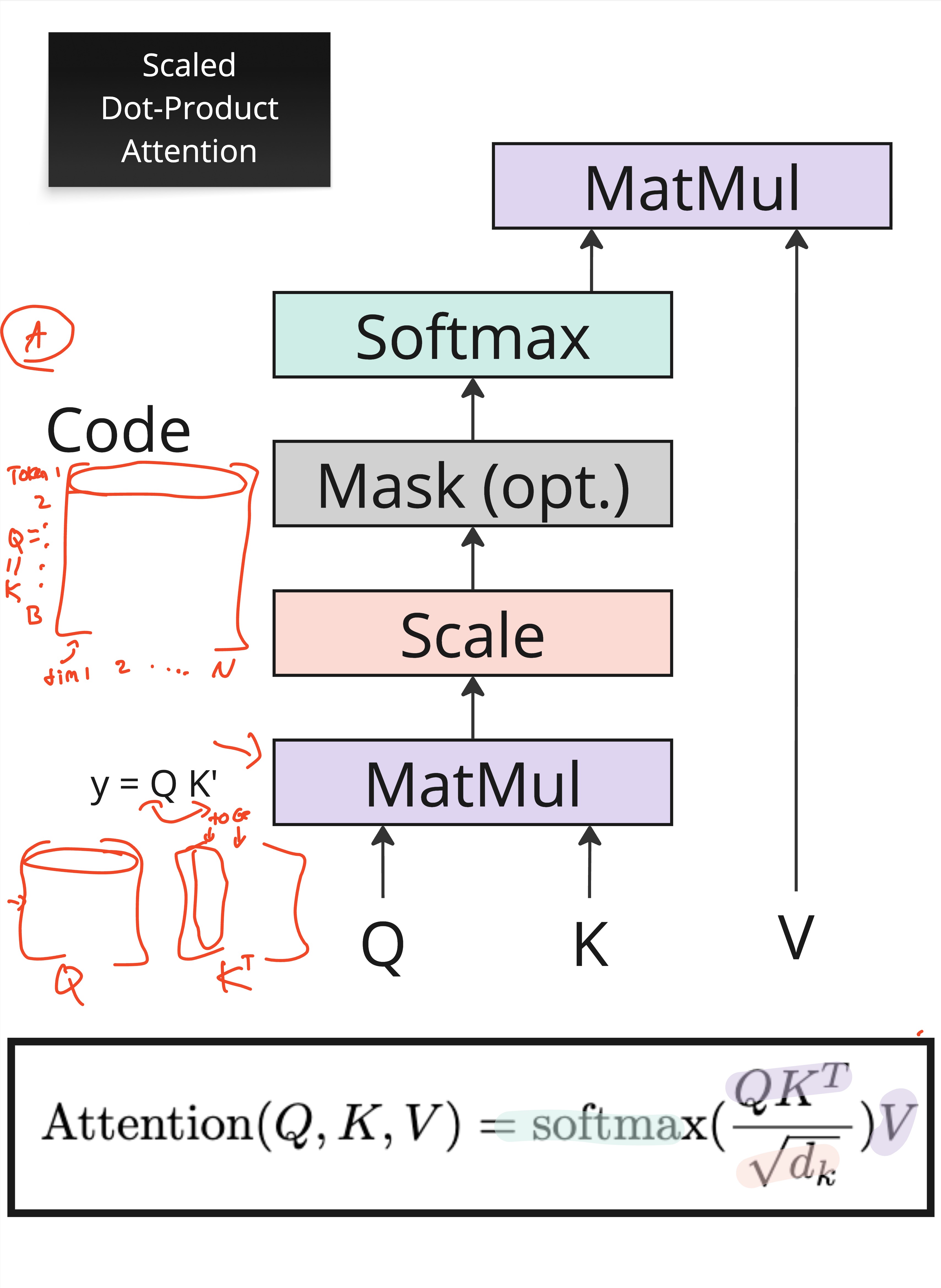
Scaled Dot-Product Attention¶

The fundamental attention computation in a Transformer is called scaled dot-product attention. It operates on three inputs:

Query ( $Q$ ): What am I looking for?
Key ( $K$ ): What do I contain?
Value ( $V$ ): What information do I carry?

Here’s the analogy: imagine searching a library database. You type a search query ( $Q$ ). Each book has index keywords ( $K$ ). When you find a match, you retrieve the book’s content ( $V$ ). Attention works the same way — the query “asks a question,” the keys determine relevance, and the values provide the answer.

The Formula¶

The complete scaled dot-product attention is computed as:

\text{Attention}(Q, K, V) = \text{softmax}\left(\frac{QK^T}{\sqrt{d_k}}\right)V

(4)

Let’s unpack this step by step:

Compute similarity scores: $QK^T$ — the dot product between each query and every key. If a query and key are similar (pointing in the same direction), the dot product is large.
Scale: Divide by $\sqrt{d_k}$ — where $d_k$ is the dimension of the key vectors. We’ll explain why shortly.
Normalize: Apply softmax to convert scores into weights that sum to 1.
Aggregate: Multiply the weights by $V$ to get a weighted combination of values.

Where Do Q, K, and V Come From?¶

In self-attention, Q, K, and V all come from the same input sequence $X$ . Each token’s embedding is projected through three separate learned linear transformations:

Q = XW^Q, \quad K = XW^K, \quad V = XW^V

(5)

The weight matrices $W^Q$ , $W^K$ , and $W^V$ are learned parameters. This is crucial: the model learns different projections for queries, keys, and values, allowing it to decouple “what I’m looking for” from “what I advertise” from “what information I carry.”

A Concrete Example¶

Let’s compute attention step by step with a tiny example.

torch.manual_seed(42)

# Suppose we have a sequence of 4 tokens, each with embedding dimension 8
seq_len, d_model = 4, 8
X = torch.randn(seq_len, d_model)

# Learned projection matrices (in practice, these are nn.Linear layers)
d_k = 4  # dimension for queries and keys
d_v = 4  # dimension for values

W_Q = torch.randn(d_model, d_k)
W_K = torch.randn(d_model, d_k)
W_V = torch.randn(d_model, d_v)

# Project input to get Q, K, V
Q = X @ W_Q  # shape: (4, 4)
K = X @ W_K  # shape: (4, 4)
V = X @ W_V  # shape: (4, 4)

print(f"Q shape: {Q.shape}")
print(f"K shape: {K.shape}")
print(f"V shape: {V.shape}")

Q shape: torch.Size([4, 4])
K shape: torch.Size([4, 4])
V shape: torch.Size([4, 4])

import math

# Step 1: Compute raw attention scores
scores = Q @ K.T  # shape: (4, 4) — score for every (query, key) pair
print("Raw scores:")
print(scores.round(decimals=2))

# Step 2: Scale by sqrt(d_k)
scaled_scores = scores / math.sqrt(d_k)
print(f"\nScaled scores (÷ √{d_k} = {math.sqrt(d_k):.1f}):")
print(scaled_scores.round(decimals=2))

# Step 3: Softmax to get attention weights
weights = F.softmax(scaled_scores, dim=-1)
print("\nAttention weights (each row sums to 1):")
print(weights.round(decimals=2))
print(f"Row sums: {weights.sum(dim=-1).tolist()}")

# Step 4: Weighted combination of values
output = weights @ V  # shape: (4, 4)
print(f"\nOutput shape: {output.shape}")

Raw scores:
tensor([[-21.8500,  22.3100,  34.1100,   5.9500],
        [ 18.5300, -18.0300,  18.3700,   6.7700],
        [  8.1200,  16.0600, -16.8700,   3.2000],
        [ -6.8400,   7.4600, -21.7400,  -4.2900]])

Scaled scores (÷ √4 = 2.0):
tensor([[-10.9300,  11.1600,  17.0600,   2.9800],
        [  9.2600,  -9.0100,   9.1900,   3.3900],
        [  4.0600,   8.0300,  -8.4400,   1.6000],
        [ -3.4200,   3.7300, -10.8700,  -2.1400]])

Attention weights (each row sums to 1):
tensor([[0.0000, 0.0000, 1.0000, 0.0000],
        [0.5200, 0.0000, 0.4800, 0.0000],
        [0.0200, 0.9800, 0.0000, 0.0000],
        [0.0000, 1.0000, 0.0000, 0.0000]])
Row sums: [1.0, 1.0, 0.9999998211860657, 1.0]

Output shape: torch.Size([4, 4])

Each row of the output is a weighted combination of the value vectors. Token 0’s output is mostly influenced by whichever tokens had the highest attention weights in row 0.

Why Scale? The $\sqrt{d_k}$ Factor¶

You might wonder: why divide by $\sqrt{d_k}$ ? Can’t we just use the raw dot products?

The issue is that as $d_k$ grows, dot products tend to grow in magnitude. When the values going into softmax are large, the output becomes extremely “spiky” — almost all the probability mass concentrates on a single element. This makes gradients very small (the softmax saturates), which cripples learning.

Dividing by $\sqrt{d_k}$ keeps the variance of the dot products roughly at 1, regardless of the dimension. This produces a diffuse distribution where the model can meaningfully spread attention across multiple tokens.

Let’s see this effect in action:

# Demonstrate the effect of scaling on softmax
sx = torch.tensor([0.1, -0.2, 0.3, -0.2, 0.5])
x = sx * 8  # Scale up to simulate large dot products

soft_x = F.softmax(x, dim=-1)
soft_sx = F.softmax(sx, dim=-1)

print(f"Large values:  softmax({x.tolist()})  = {soft_x.tolist()}")
print(f"Small values:  softmax({sx.tolist()}) = {soft_sx.tolist()}")

fig, ax = plt.subplots(figsize=(6, 3))
positions = range(len(sx))
width = 0.35
ax.bar([p - width/2 for p in positions], soft_x.tolist(), width, label="softmax(x) — unscaled", color="salmon")
ax.bar([p + width/2 for p in positions], soft_sx.tolist(), width, label="softmax(sx) — scaled", color="steelblue")
ax.set_xlabel("Position")
ax.set_ylabel("Probability")
ax.set_title("Scaling prevents spiky attention distributions")
ax.legend()
plt.tight_layout()
plt.show()

Large values:  softmax([0.800000011920929, -1.600000023841858, 2.4000000953674316, -1.600000023841858, 4.0])  = [0.03260834142565727, 0.002958162222057581, 0.1615101844072342, 0.002958162222057581, 0.7999651432037354]
Small values:  softmax([0.10000000149011612, -0.20000000298023224, 0.30000001192092896, -0.20000000298023224, 0.5]) = [0.19249781966209412, 0.14260590076446533, 0.2351173758506775, 0.14260590076446533, 0.28717300295829773]

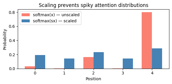
The orange bars (unscaled) are extremely spiky — almost all attention goes to position 4. The blue bars (scaled) spread attention more evenly, allowing the model to attend to multiple positions simultaneously.

Exercise 6.1: Attention Score Computation

Suppose we have a sequence of three tokens with query and key dimension $d_k = 2$ . The Q and K matrices are:

Q = \begin{bmatrix} 1 & 0 \\ 0 & 1 \\ 1 & 1 \end{bmatrix}, \quad K = \begin{bmatrix} 1 & 0 \\ 0 & 1 \\ 0.5 & 0.5 \end{bmatrix}

(6)

(a) Compute the raw attention score matrix $QK^T$ .

(b) Apply scaling by $\sqrt{d_k}$ .

(c) Apply softmax row-wise to get the attention weights. Which token does token 3 (row 3) attend to most equally? Why does this make sense given its query vector $[1, 1]$ ?

# You can verify your answers with:
import torch
import torch.nn.functional as F
import math

Q = torch.tensor([[1., 0.], [0., 1.], [1., 1.]])
K = torch.tensor([[1., 0.], [0., 1.], [0.5, 0.5]])

scores = Q @ K.T
scaled = scores / math.sqrt(2)
weights = F.softmax(scaled, dim=-1)
print("Weights:", weights.round(decimals=3))

Masking: Controlling What Attention Can See¶

In some settings, we need to prevent attention from looking at certain positions. The most important case is in the decoder during generation: when predicting the next token, the model should only attend to previous tokens, not future ones. (Otherwise, it would be “cheating” by peeking at the answer.)

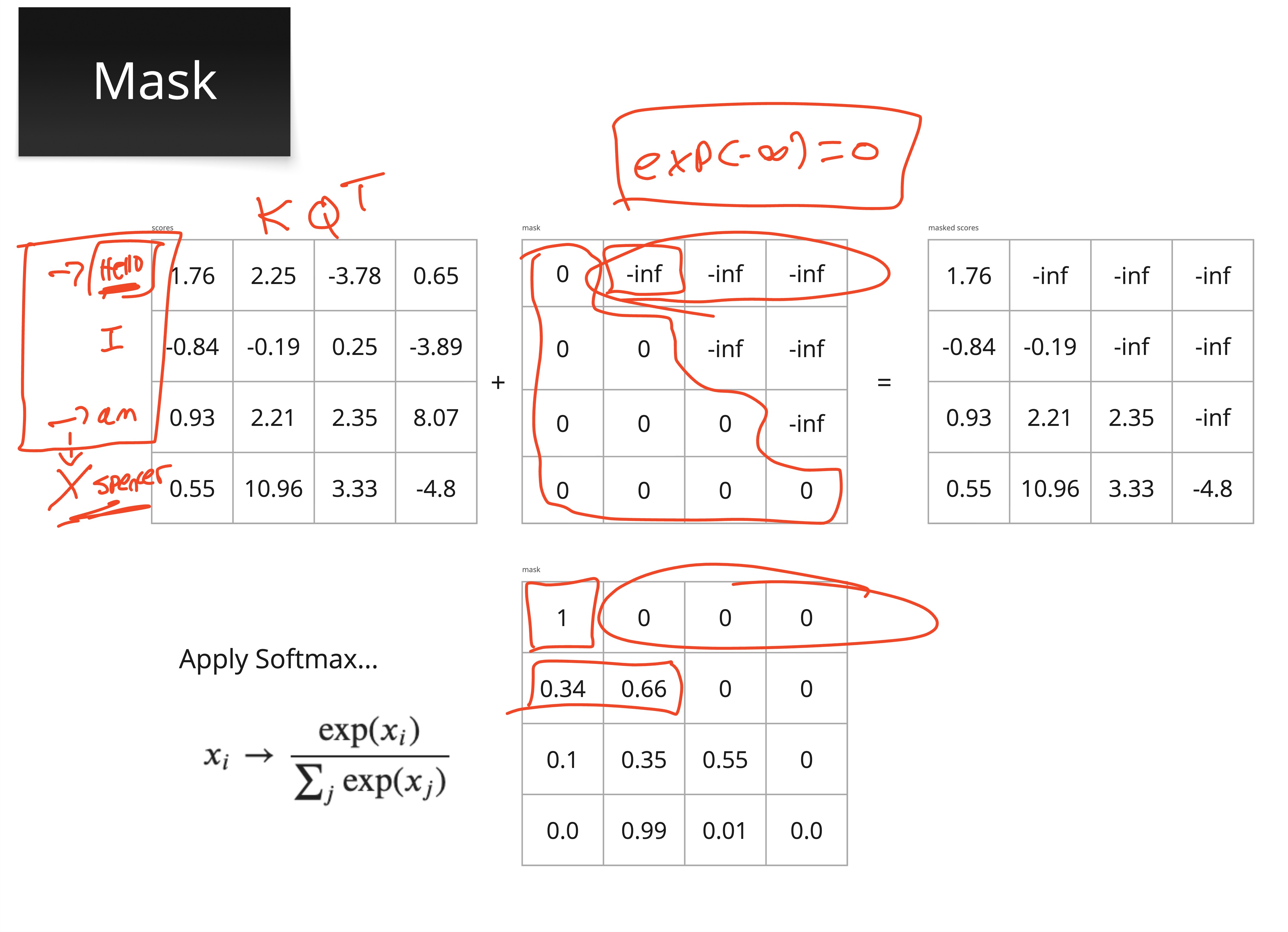
This is achieved with a causal mask — a lower-triangular matrix of zeros and negative infinities:

\text{mask} = \begin{bmatrix} 0 & -\infty & -\infty & -\infty \\ 0 & 0 & -\infty & -\infty \\ 0 & 0 & 0 & -\infty \\ 0 & 0 & 0 & 0 \end{bmatrix}

(7)

We add this mask to the scaled attention scores before applying softmax. Since $\exp(-\infty) = 0$ , masked positions get zero attention weight — they’re completely invisible.

Let’s see this in action with a concrete example:

# Example: "Hello I am Spencer" — 4 tokens
tokens = ["Hello", "I", "am", "Spencer"]

torch.manual_seed(0)
scores = torch.randn(4, 4)  # Pretend these are our QK^T scores

# Create causal mask: upper triangle is -inf
mask = torch.triu(torch.ones(4, 4) * float('-inf'), diagonal=1)
print("Causal mask:")
print(mask)

# Apply mask
masked_scores = scores + mask
print("\nMasked scores:")
print(masked_scores.round(decimals=2))

# Softmax — masked positions become 0
weights = F.softmax(masked_scores, dim=-1)
print("\nAttention weights (causal):")
for i, token in enumerate(tokens):
    row = [f"{w:.2f}" for w in weights[i].tolist()]
    print(f"  {token:>8s} attends to: {row}")

Causal mask:
tensor([[0., -inf, -inf, -inf],
        [0., 0., -inf, -inf],
        [0., 0., 0., -inf],
        [0., 0., 0., 0.]])

Masked scores:
tensor([[-1.1300,    -inf,    -inf,    -inf],
        [ 0.8500,  0.6900,    -inf,    -inf],
        [ 0.3200, -1.2600,  0.3500,    -inf],
        [ 0.1200,  1.2400,  1.1200, -0.2500]])

Attention weights (causal):
     Hello attends to: ['1.00', '0.00', '0.00', '0.00']
         I attends to: ['0.54', '0.46', '0.00', '0.00']
        am attends to: ['0.45', '0.09', '0.46', '0.00']
   Spencer attends to: ['0.13', '0.41', '0.36', '0.09']

Notice the pattern: “Hello” can only attend to itself. “I” can attend to “Hello” and itself. “Spencer” can attend to all four tokens. This ensures the model never “peeks” at future tokens during generation.

Multi-Head Attention¶

A single attention head computes one set of attention weights — one “perspective” on the relationships between tokens. But language has many simultaneous relationships: syntactic structure, semantic similarity, coreference, proximity, and more.

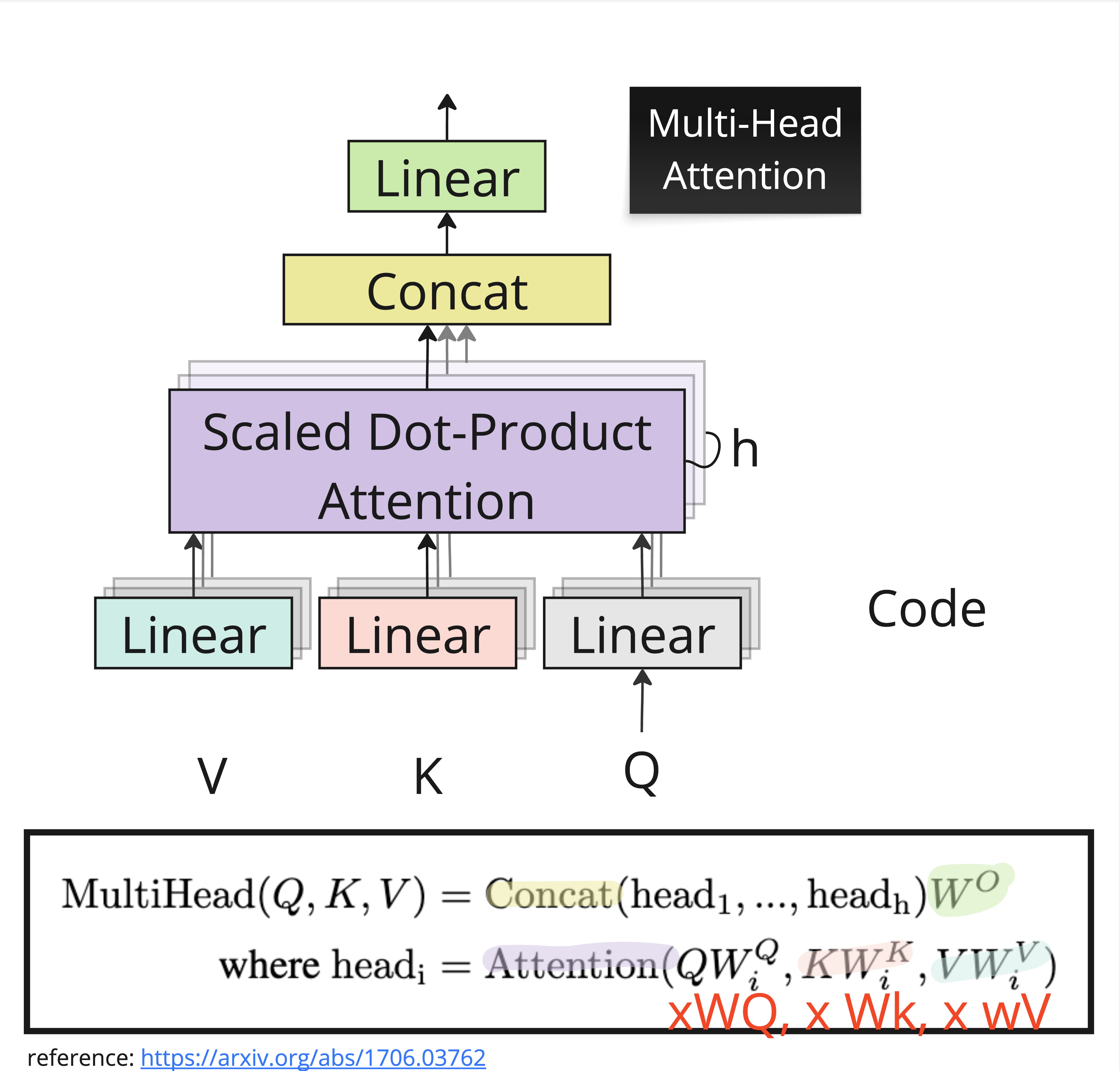
Multi-head attention runs $h$ attention heads in parallel, each with its own learned projections $W_i^Q$ , $W_i^K$ , $W_i^V$ . Each head can learn to focus on a different type of relationship. The outputs are then concatenated and projected through a final linear layer:

\text{MultiHead}(Q, K, V) = \text{Concat}(\text{head}_1, \ldots, \text{head}_h) \, W^O

(8)

where each head is:

\text{head}_i = \text{Attention}(QW_i^Q, \, KW_i^K, \, VW_i^V)

(9)

The Shape Trick¶

An important implementation detail: if the model dimension is $d_{\text{model}}$ and we have $h$ heads, each head operates on dimension $d_k = d_{\text{model}} / h$ . So multi-head attention doesn’t increase the computational cost compared to a single head with the full dimension — it just splits the representation into $h$ subspaces.

For example, with $d_{\text{model}} = 512$ and $h = 8$ heads, each head works with $d_k = 64$ dimensions. The concatenation of all 8 heads produces a 512-dimensional output, which then goes through $W^O$ back to $d_{\text{model}}$ .

# Multi-head attention: split d_model into h heads
d_model = 512
n_heads = 8
d_k = d_model // n_heads

print(f"Model dimension: {d_model}")
print(f"Number of heads: {n_heads}")
print(f"Per-head dimension: {d_k}")
print(f"After concat: {n_heads} × {d_k} = {n_heads * d_k} (back to d_model)")

Model dimension: 512
Number of heads: 8
Per-head dimension: 64
After concat: 8 × 64 = 512 (back to d_model)

# PyTorch provides MultiheadAttention out of the box
mha = nn.MultiheadAttention(embed_dim=d_model, num_heads=n_heads, batch_first=True)

# Count parameters
total_params = sum(p.numel() for p in mha.parameters())
print(f"Total parameters in MultiheadAttention: {total_params:,}")
print(f"  W_Q, W_K, W_V: 3 × ({d_model} × {d_model}) = {3 * d_model * d_model:,}")
print(f"  W_O: {d_model} × {d_model} = {d_model * d_model:,}")
print(f"  + biases: {4 * d_model:,}")

Total parameters in MultiheadAttention: 1,050,624
  W_Q, W_K, W_V: 3 × (512 × 512) = 786,432
  W_O: 512 × 512 = 262,144
  + biases: 2,048

Putting It Together: The Transformer Block¶

Now that we understand attention, let’s see how it fits into the broader architecture. A Transformer block wraps attention with three additional components: residual connections, layer normalization, and a feed-forward network. Let’s examine each one.

Residual Connections¶

Deep networks are hard to train. As we stack more layers, gradients must travel through every layer during backpropagation — and they can shrink or explode along the way (the vanishing gradient problem we saw with RNNs).

Residual connections (also called skip connections) provide a simple but powerful fix. Instead of computing:

x \rightarrow f(x)

(10)

We compute:

x \rightarrow x + f(x)

(11)

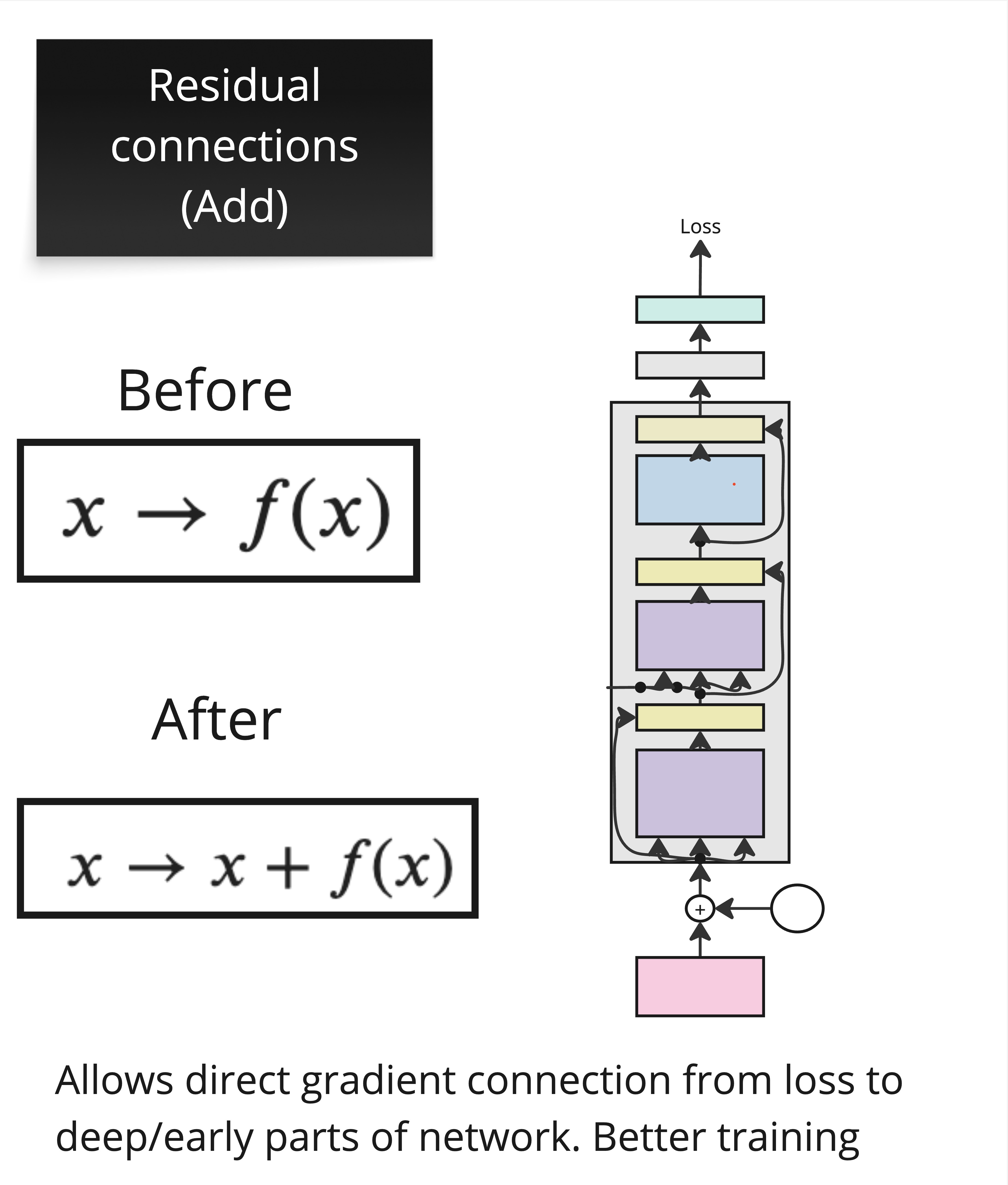
The input $x$ is added directly to the output of the sublayer. This creates a “gradient highway” — during backpropagation, the gradient can flow directly through the addition, bypassing the potentially gradient-shrinking sublayer. The sublayer only needs to learn the residual — how to modify the input, not reconstruct it from scratch.

In the Transformer, every sublayer (attention and feed-forward) uses a residual connection.

Layer Normalization¶

Layer normalization normalizes the features for each individual token, producing mean 0 and standard deviation 1. It then applies learned scale ( $\gamma$ ) and shift ( $\beta$ ) parameters:

\text{LayerNorm}(x) = \frac{x - E(x)}{\sqrt{\text{var}(x) + \epsilon}} \cdot \gamma + \beta

(12)

Key points about layer normalization:

Applied across features (the embedding dimension) for each token independently — not across the batch or sequence
Makes all features have mean 0 and standard deviation 1, preventing any single feature from dominating
The learnable parameters $\gamma$ and $\beta$ allow the network to undo the normalization if needed
Stabilizes training by keeping activations in a well-behaved range

An interesting detail: the original paper applied layer norm after each sublayer (post-norm), but modern Transformers typically apply it before (pre-norm). Pre-norm tends to train more stably, especially for very deep models.

# Layer normalization in action
d_model = 8
layer_norm = nn.LayerNorm(d_model)

# A single token's feature vector
x = torch.tensor([5.0, -3.0, 1.0, 0.5, -1.0, 2.0, 8.0, -2.0])
normed = layer_norm(x)

print(f"Input:      {x.tolist()}")
print(f"  mean={x.mean():.2f}, std={x.std():.2f}")
print(f"Normalized: {normed.data.tolist()}")
print(f"  mean={normed.data.mean():.4f}, std={normed.data.std():.2f}")

Input:      [5.0, -3.0, 1.0, 0.5, -1.0, 2.0, 8.0, -2.0]
  mean=1.31, std=3.67
Normalized: [1.073081612586975, -1.2549599409103394, -0.09093915671110153, -0.23644176125526428, -0.672949492931366, 0.20006603002548218, 1.9460972547531128, -0.9639546871185303]
  mean=-0.0000, std=1.07

Position-wise Feed-Forward Network¶

After attention gathers information from across the sequence, each token passes through a feed-forward network (FFN) independently. This is a simple two-layer network with a ReLU activation:

\text{FFN}(x) = \max(0, \; xW_1 + b_1) \, W_2 + b_2

(13)

The “position-wise” name means the same feed-forward network is applied independently to each token position — there’s no interaction between tokens here. (That’s attention’s job.)

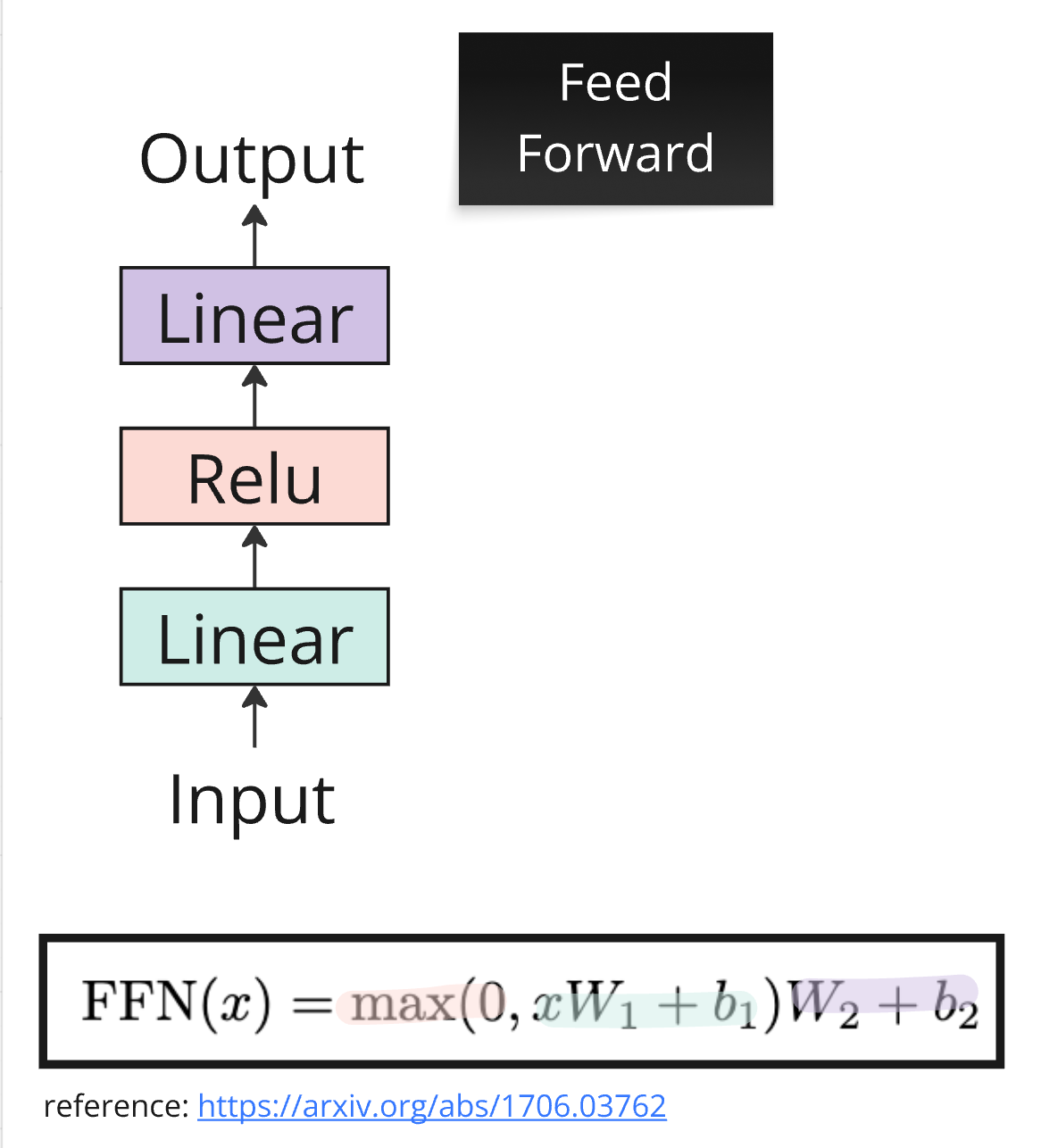
A key design choice: the inner dimension is typically 4x the model dimension. So if $d_{\text{model}} = 512$ , the hidden layer has dimension 2048. This expansion gives the network more capacity to transform each token’s representation.

# The feed-forward network from the paper
class FeedForward(nn.Module):
    def __init__(self, d_model):
        super().__init__()
        self.net = nn.Sequential(
            nn.Linear(d_model, 4 * d_model),  # Expand to 4x
            nn.ReLU(),
            nn.Linear(4 * d_model, d_model),  # Project back
        )

    def forward(self, x):
        return self.net(x)

ffn = FeedForward(512)
n_params = sum(p.numel() for p in ffn.parameters())
print(f"FFN parameters: {n_params:,}")
print(f"  Layer 1: 512 × 2048 + 2048 bias = {512*2048 + 2048:,}")
print(f"  Layer 2: 2048 × 512 + 512 bias = {2048*512 + 512:,}")

FFN parameters: 2,099,712
  Layer 1: 512 × 2048 + 2048 bias = 1,050,624
  Layer 2: 2048 × 512 + 512 bias = 1,049,088

Putting the Block Together¶

A complete Transformer block chains these components with residual connections and layer norm:

Self-Attention sublayer: x = x + MultiHeadAttention(LayerNorm(x))
Feed-Forward sublayer: x = x + FeedForward(LayerNorm(x))

The full Transformer stacks $N$ of these identical blocks. The original paper used $N = 6$ , but modern models use many more (GPT-3 uses 96 blocks!).

Positional Encoding¶

There’s a problem we haven’t addressed yet. Attention treats its input as a set, not a sequence — it computes all pairwise interactions without any notion of order. If we shuffled the tokens, the attention scores would be different (because the inputs changed), but the architecture itself has no way to know that “the” at position 1 is different from “the” at position 10.

This is fundamentally different from RNNs and CNNs, which have position built into their structure (RNNs process tokens left-to-right; CNNs use local windows).

Transformers solve this with positional encoding — adding positional information to the input embeddings. The original paper used sinusoidal functions with different frequencies:

PE_{(pos, 2i)} = \sin\left(\frac{pos}{10000^{2i / d_{\text{model}}}}\right)

(14)

PE_{(pos, 2i+1)} = \cos\left(\frac{pos}{10000^{2i / d_{\text{model}}}}\right)

(15)

where $pos$ is the position in the sequence and $i$ is the dimension index.

Why sinusoids? Several nice properties:

Cyclical: The encoding naturally handles relative positions — the model can learn to attend to “3 positions back” because the relationship between $PE_{pos}$ and $PE_{pos+3}$ is consistent
Extrapolation: Can handle sequences longer than any seen during training
Data-independent: Depends only on position, not on the content

import numpy as np

def positional_encoding(max_len, d_model, n=10000):
    """Compute sinusoidal positional encoding."""
    PE = np.zeros((max_len, d_model))
    for pos in range(max_len):
        for i in range(d_model // 2):
            x = pos / (n ** (2 * i / d_model))
            PE[pos, 2*i] = np.sin(x)
            PE[pos, 2*i + 1] = np.cos(x)
    return PE

PE = positional_encoding(50, 64)

fig, ax = plt.subplots(figsize=(8, 4))
im = ax.imshow(PE.T, aspect='auto', cmap='RdBu')
ax.set_xlabel("Position in sequence")
ax.set_ylabel("Embedding dimension")
ax.set_title("Sinusoidal Positional Encoding")
plt.colorbar(im, ax=ax)
plt.tight_layout()
plt.show()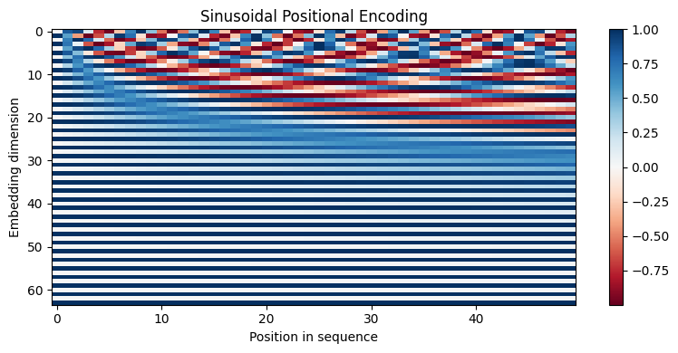

Each column is a position vector that gets added to the corresponding token embedding. The lower dimensions oscillate quickly (high frequency), while higher dimensions oscillate slowly (low frequency). This multi-scale pattern gives the model access to both fine-grained and coarse-grained positional information.

In practice, many modern Transformers replace sinusoidal encodings with learned positional embeddings — a simple nn.Embedding layer that treats each position as a learnable vector. This works well when the maximum sequence length is fixed during training.

Computational Considerations¶

The Transformer’s power comes at a cost. The self-attention mechanism computes dot products between every pair of tokens, making its time and memory complexity quadratic in the sequence length:

O(n^2 \cdot d)

(16)

where $n$ is the sequence length and $d$ is the model dimension. For a sequence of 1,000 tokens, that’s 1 million pairwise scores per attention head per layer.

This quadratic scaling is the main bottleneck for processing very long documents. It’s why models have context windows — maximum sequence lengths they can handle (e.g., 4K, 8K, 128K tokens). Research on efficient attention variants (sparse attention, linear attention, flash attention) aims to push these limits further.

Wrap-Up¶

Key Takeaways¶

Key Takeaways

Transformers replace recurrence with attention, processing all tokens in parallel and enabling direct connections between any positions in a sequence
Scaled dot-product attention computes relevance between queries and keys ( $QK^T / \sqrt{d_k}$ ), normalizes with softmax, and produces a weighted combination of values — the scaling factor prevents softmax saturation
Queries, keys, and values are learned linear projections of the input — the model learns to separate “what I’m looking for” ( $Q$ ) from “what I advertise” ( $K$ ) from “what information I carry” ( $V$ )
Multi-head attention runs $h$ parallel attention operations, allowing the model to simultaneously attend to different types of relationships (syntax, semantics, coreference, etc.)
Causal masking prevents the decoder from attending to future tokens by adding $-\infty$ to the upper triangle of attention scores, ensuring autoregressive generation
Residual connections and layer normalization enable stable training of deep Transformer stacks by providing gradient highways and keeping activations well-scaled
Positional encoding injects sequence order information that the attention mechanism lacks, using either sinusoidal functions or learned embeddings

What’s Next¶

In Part 02, we’ll get hands-on with PyTorch and build the Transformer’s components from scratch. You’ll implement scaled dot-product attention, multi-head attention, and a complete Transformer block step by step — then visualize attention patterns on real text to see what the model learns to attend to. With the conceptual foundation from this lecture, you’ll understand exactly what each line of code is doing and why.