Transformer Model Variants
CAP-6640: Computational Understanding of Natural Language
Spencer Lyon
Prerequisites
L06.01: The Transformer architecture — self-attention, multi-head attention, positional encoding, masking, and transformer blocks
L06.02: Attention from Scratch — hands-on implementation in PyTorch
Outcomes
Compare the three major transformer variants (encoder-only, decoder-only, encoder-decoder) in terms of attention patterns, pretraining objectives, and task alignment
Explain masked language modeling and how bidirectional context enables understanding tasks
Explain causal language modeling and how autoregressive generation works in decoder-only models
Describe how encoder-decoder models combine both mechanisms for sequence-to-sequence tasks
Select the appropriate architecture variant for a given NLP task and justify the choice
References
Devlin et al. (2018) — BERT: Pre-training of Deep Bidirectional Transformers
Liu et al. (2019) — RoBERTa: A Robustly Optimized BERT Pretraining Approach
Raffel et al. (2020) — T5: Exploring the Limits of Transfer Learning
Kaplan et al. (2020) — Scaling Laws for Neural Language Models
One Architecture, Three Philosophies
Last week, we built the Transformer from the ground up — self-attention, multi-head attention, residual connections, the works. The original Transformer was designed for machine translation, and it used both an encoder and a decoder working together.
But here’s the thing: BERT doesn’t have a decoder. GPT doesn’t have an encoder. T5 uses both. Yet all three are called “Transformers.” How can that be?
The answer is surprisingly simple. The original Transformer has two halves, and researchers discovered that you can take either half (or both) and pretrain it on a massive corpus to create a powerful language model. The choice of which half you use determines what your model is naturally good at:
Use only the encoder → a model that excels at understanding text (classification, NER, similarity)
Use only the decoder → a model that excels at generating text (completions, conversations, creative writing)
Use both → a model that excels at transforming one text into another (translation, summarization)
This lecture explores each of these three families. We’ll see how a single architectural choice — which half of the Transformer you keep, and what you mask — leads to fundamentally different capabilities.

Figure 1:The original Transformer splits into three model families, each defined by which components are kept and what pretraining objective is used.
import torch
import torch.nn.functional as F
import matplotlib.pyplot as plt
import matplotlib.patches as mpatches
Encoder-Only Models
The Key Idea: Bidirectional Context
Recall from Week 6 that the encoder side of the Transformer uses bidirectional attention — every token can attend to every other token in the sequence. There is no causal mask. When processing the word “bank” in “I sat by the river bank,” the model sees both the left context (“I sat by the river”) and the right context simultaneously. This is incredibly powerful for tasks that require understanding the meaning of text.
Encoder-only models take just this encoder stack and throw away the decoder entirely. The result is a model that builds rich, contextual representations of input text — representations that capture meaning in both directions.
But here’s a problem: if the model can see everything at once, how do we train it? We can’t use next-token prediction because the model would simply look ahead and copy the answer. We need a different pretraining objective.
Masked Language Modeling
The solution is Masked Language Modeling — a clever “fill-in-the-blank” game. During training, we randomly mask out about 15% of the tokens in each input and ask the model to predict them from the surrounding context.
For example, given the input:
“The cat [MASK] on the [MASK] because it was tired”
The model must predict that the first blank is “sat” and the second is “mat” — using all the surrounding context from both directions. This forces the model to build deep, bidirectional representations that capture the relationships between words.
![Each [MASK] token is predicted using context from both directions — the hallmark of encoder-only pretraining.](/build/mlm_pretraining-a64e71a91eb05e052d4f671f4106bf9a.svg)
Figure 2:Each [MASK] token is predicted using context from both directions — the hallmark of encoder-only pretraining.
Let’s visualize the difference between the attention patterns. In the encoder, every token sees every other token. Compare this with the causal mask we saw last week, where each token can only see tokens that came before it:
fig, axes = plt.subplots(1, 2, figsize=(10, 4))

seq_len = 5
tokens = ["The", "cat", "sat", "on", "mat"]

# Encoder-only: bidirectional (full attention)
bidir_mask = torch.ones(seq_len, seq_len)
axes[0].imshow(bidir_mask, cmap="Blues", vmin=0, vmax=1)
axes[0].set_title("Encoder-Only\n(Bidirectional)", fontsize=13)
axes[0].set_xticks(range(seq_len))
axes[0].set_yticks(range(seq_len))
axes[0].set_xticklabels(tokens, fontsize=10)
axes[0].set_yticklabels(tokens, fontsize=10)
axes[0].set_xlabel("Attends to")
axes[0].set_ylabel("Token")

# Decoder-only: causal (lower triangular)
causal_mask = torch.tril(torch.ones(seq_len, seq_len))
axes[1].imshow(causal_mask, cmap="Oranges", vmin=0, vmax=1)
axes[1].set_title("Decoder-Only\n(Causal)", fontsize=13)
axes[1].set_xticks(range(seq_len))
axes[1].set_yticks(range(seq_len))
axes[1].set_xticklabels(tokens, fontsize=10)
axes[1].set_yticklabels(tokens, fontsize=10)
axes[1].set_xlabel("Attends to")
axes[1].set_ylabel("Token")

plt.tight_layout()
plt.show()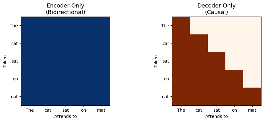
The blue grid on the left is all ones — every token can attend to every other token. The orange triangular matrix on the right enforces causal ordering — token can only attend to tokens .
This single difference — the shape of the attention mask — is what separates the two model families.
From BERT to RoBERTa
The first major encoder-only model was BERT (Bidirectional Encoder Representations from Transformers), published by Devlin et al. at Google in 2018. BERT was a landmark result: it achieved state-of-the-art on 11 NLP benchmarks simultaneously, and it demonstrated the power of bidirectional pretraining.
BERT came in two sizes:
| Model | Layers | Hidden Size | Attention Heads | Parameters |
|---|---|---|---|---|
| BERT-base | 12 | 768 | 12 | 110M |
| BERT-large | 24 | 1024 | 16 | 340M |
BERT’s pretraining used two objectives: Masked Language Modeling (MLM) and Next Sentence Prediction (NSP). The NSP task trained the model to predict whether two sentences appeared consecutively in the original text. The idea was to help BERT understand relationships between sentences.
However, subsequent research found that BERT’s recipe could be significantly improved. In 2019, Liu et al. published RoBERTa (Robustly Optimized BERT Pretraining Approach), which kept BERT’s architecture but made several training improvements:
Dropped the NSP objective — it turned out to be unnecessary, and even slightly harmful
Trained on more data — 160GB vs. BERT’s 16GB of text
Trained for longer — more steps with larger batches
Dynamic masking — instead of masking the same tokens every epoch, the masking pattern changes each time the model sees a sequence
The result? RoBERTa matched or exceeded BERT’s performance on every benchmark, demonstrating that BERT was significantly undertrained. This makes RoBERTa the canonical encoder-only model we reference today.
What Encoder-Only Models Excel At
Because encoder-only models build bidirectional representations, they are naturally suited for tasks that require understanding the full context of a piece of text:
Text classification — sentiment analysis, spam detection, topic labeling (use the [CLS] token representation as input to a classification head)
Named Entity Recognition — label each token as person, organization, location, etc. (use per-token representations)
Extractive Question Answering — given a question and a passage, identify the span of text that answers the question (predict start and end positions)
Semantic similarity — determine how similar two sentences are (compare their [CLS] representations)
What they cannot do well is generate text. Because the model sees all positions simultaneously during training, it has no natural mechanism for producing tokens one at a time. You can’t ask RoBERTa to “continue this sentence” — it was trained to fill in blanks, not to write left to right.
Decoder-Only Models
The Key Idea: Causal Language Modeling
Decoder-only models take the opposite approach: they use only the decoder stack with causal masking, where each token can only attend to itself and all preceding tokens. This is the same lower-triangular mask we studied in Week 6.
The pretraining objective is causal language modeling — predicting the next token given all previous tokens. Given a sequence of tokens , the model learns to predict:
for every position in the sequence. This is the classic language modeling task, the same one that N-gram models attempted decades ago — but now powered by the full expressiveness of the Transformer architecture.

Figure 3:Each token predicts the next token using only left context — the hallmark of decoder-only pretraining.
The GPT Lineage
The decoder-only story begins with GPT (Generative Pre-trained Transformer), published by Radford et al. at OpenAI in 2018 — the same year as BERT. The two papers represented competing bets on which half of the Transformer would prove more useful.
The GPT lineage tracks the rapid scaling of decoder-only models:
| Model | Year | Parameters | Key Innovation |
|---|---|---|---|
| GPT | 2018 | 117M | Showed that pretraining a decoder works for downstream tasks |
| GPT-2 | 2019 | 1.5B | Demonstrated coherent long-form text generation |
| GPT-3 | 2020 | 175B | Discovered in-context learning and few-shot prompting |
| GPT-4 | 2023 | Undisclosed | Multimodal input, advanced reasoning |
Each generation grew dramatically in scale, and with that scale came qualitatively new capabilities. GPT-3 was particularly significant because it showed that a sufficiently large decoder-only model could perform tasks it was never explicitly trained for — simply by providing a few examples in the prompt. This in-context learning ability changed the field overnight.

Figure 4:The rapid scaling of decoder-only models from GPT (117M parameters) to GPT-4, with qualitatively new capabilities emerging at each scale.
Why Causal Masking Enables Generation
The beauty of causal masking is that it makes generation trivially straightforward. During training, the model learns to predict each next token from its predecessors. At inference time, we can generate text by:
Feed in a prompt:
The model predicts a distribution over the next token:
Sample or pick the most likely token
Append it to the sequence and repeat
This autoregressive process generates text one token at a time, and it works seamlessly because the model was trained in exactly this left-to-right fashion.
The Surprising Discovery: Understanding Through Generation
Here’s what caught the field by surprise: with enough scale, decoder-only models can also understand text. GPT-3 showed that you can do text classification, NER, translation, and many other “understanding” tasks simply by framing them as text generation problems.
Want sentiment analysis? Just prompt the model:
“Review: This movie was fantastic! Sentiment:”
And the model generates “Positive.” No fine-tuning needed — just a well-crafted prompt.
This prompt-based approach to NLP tasks is why decoder-only models have become so dominant. Instead of needing separate, fine-tuned models for each task (as with BERT/RoBERTa), a single large decoder-only model can handle almost anything through appropriate prompting. Models like GPT-4, Claude, and LLaMA are all decoder-only Transformers.
Why Decoder-Only Won (So Far)
The dominance of decoder-only models is one of the most important developments in modern NLP — and it wasn’t obvious in advance. In 2018, BERT and GPT were published in the same year, representing competing bets on which half of the Transformer mattered more. BERT won the initial benchmarks convincingly. But within five years, the field had decisively shifted to decoder-only. Why?
Several factors converged:
Training signal density. This is perhaps the most fundamental advantage. In causal language modeling, every token in the training data provides a learning signal — the model must predict token from tokens . With MLM (the encoder-only objective), only the ~15% of randomly masked tokens contribute to the loss. The remaining 85% provide context but don’t directly drive weight updates. For the same training data, a decoder-only model extracts roughly 6–7x more gradient signal per pass through the corpus. When you’re training on trillions of tokens, that efficiency gap is enormous.
Predictable scaling. In 2020, Kaplan et al. at OpenAI discovered that decoder-only model performance follows remarkably clean power laws: as you increase model size, dataset size, or compute, the loss decreases along smooth, predictable curves. This was transformative — it meant labs could invest billions of dollars in larger models with reasonable confidence about the outcome. These scaling laws weren’t established for encoder-only or encoder-decoder models at comparable scales, so investment naturally concentrated on the architecture with the clearest roadmap.
The output bottleneck of encoders. Consider what happens when you scale an encoder-only model to 175B parameters. Its output is still a fixed-dimensional vector — a 768- or 1024-dimensional [CLS] representation — that must be routed through a small, task-specific classification head. Even a massive encoder can only “answer” in the limited vocabulary of that head (e.g., “positive” vs. “negative”). A decoder-only model’s output is generated text, which can express anything: labels, translations, reasoning chains, code, poetry. This means decoder-only models can demonstrate new capabilities simply by generating new kinds of text, while encoder-only models are structurally limited to the tasks their heads were designed for.
Next-token prediction is a harder (and richer) objective. MLM asks: “given all the words around this blank, what word goes here?” The bidirectional context heavily constrains the answer — there’s usually only one or a few words that fit. Causal language modeling asks: “given only what came before, what comes next?” This is a fundamentally harder problem. With only left context, the model must build deeper internal models of language structure, world knowledge, and reasoning to make good predictions. It can’t “cheat” by looking at words to the right. At scale, this harder objective forces the model to develop richer internal representations.
Generation naturally supports in-context learning. When a user puts examples in a prompt, a decoder-only model processes them left-to-right, building up an internal representation of “what task is being demonstrated.” Each subsequent prediction is conditioned on all the examples that came before. This sequential conditioning is the mechanism behind in-context learning — and it simply doesn’t exist in encoder-only models, which process all tokens simultaneously and have no concept of “now generate an answer to what came before.”
Architectural simplicity. A decoder-only model is a single stack of Transformer blocks with a causal mask. No cross-attention layers, no separate encoder and decoder to coordinate. This simplicity has real engineering benefits: easier parallelization across GPUs, more straightforward inference optimization (particularly KV-caching, where previously computed key-value pairs are reused as each new token is generated), and simpler codebases to maintain and debug at scale.
These factors are mutually reinforcing. Training efficiency → more investment in scaling → scaling reveals emergent capabilities unique to the generation paradigm → more interest → more investment. By the time the field realized how powerful scaled decoder-only models could be, the gap in research attention (and funding) had become self-perpetuating.
Encoder-Decoder Models
The Key Idea: Understand Then Generate
Encoder-decoder models keep the full original Transformer architecture: an encoder that processes the input with bidirectional attention, and a decoder that generates the output autoregressively with causal masking. The two halves are connected through cross-attention — the decoder attends to the encoder’s output representations when generating each token.
This architecture is a natural fit for tasks where the input and output are different sequences. The encoder builds a rich, bidirectional understanding of the input, and the decoder uses that understanding to generate a new sequence.

Figure 5:The encoder builds bidirectional representations of the input; the decoder generates the output autoregressively, attending to the encoder’s representations via cross-attention.
T5: Everything is Text-to-Text
The most influential encoder-decoder model is T5 (Text-to-Text Transfer Transformer), published by Raffel et al. at Google in 2020. T5’s key innovation was a unifying idea: every NLP task can be framed as transforming one text string into another.
Instead of adding task-specific heads (like BERT does for classification vs. NER vs. QA), T5 prepends a task prefix to the input and generates the output as text:
| Task | Input | Output |
|---|---|---|
| Translation | “translate English to German: That is good” | “Das ist gut” |
| Summarization | “summarize: The lengthy article about...” | “Article discusses...” |
| Classification | “classify sentiment: This movie was great!” | “positive” |
| QA | “question: What is the capital? context: France’s capital is Paris.” | “Paris” |
This text-to-text framing is elegant: one model, one format, many tasks. T5 was pretrained using a variation of masked language modeling called span corruption — instead of masking individual tokens, it masks contiguous spans of text, and the model must generate the missing spans.
BART: A Denoising Perspective
Another notable encoder-decoder model is BART (Bidirectional and Auto-Regressive Transformer), published by Lewis et al. at Facebook in 2019. BART takes a different angle on pretraining: it corrupts the input text in various ways (masking, deletion, permutation, rotation) and trains the model to reconstruct the original. This denoising autoencoder approach makes BART particularly strong at text generation tasks like abstractive summarization.
When to Use Encoder-Decoder
Encoder-decoder models shine when:
The input and output are structurally different — different lengths, different languages, different formats
You need strong understanding of the input (bidirectional encoder) combined with fluent generation of the output (autoregressive decoder)
The task naturally decomposes into “read this” then “write that” — machine translation, summarization, generative QA
The trade-off is complexity: encoder-decoder models have roughly twice the parameters of a single-stack model at the same depth (because you’re maintaining two separate stacks plus cross-attention layers). As decoder-only models have grown powerful enough to handle many of these tasks through prompting alone, the practical advantages of encoder-decoder models have narrowed. But for tasks like translation, where the structural separation between input and output is clear, they remain a strong choice.
The Big Picture
Let’s bring everything together. The three Transformer variants are defined by two choices: which components of the original architecture you keep, and what pretraining objective you use.
fig, axes = plt.subplots(1, 3, figsize=(14, 4))

tokens = ["T₁", "T₂", "T₃", "T₄"]
n = len(tokens)

# Encoder-only: bidirectional
bidir = torch.ones(n, n)
axes[0].imshow(bidir, cmap="Blues", vmin=0, vmax=1.3)
axes[0].set_title("Encoder-Only\n(BERT, RoBERTa)", fontsize=12, fontweight="bold")
axes[0].set_xticks(range(n)); axes[0].set_yticks(range(n))
axes[0].set_xticklabels(tokens); axes[0].set_yticklabels(tokens)

# Decoder-only: causal
causal = torch.tril(torch.ones(n, n))
im2 = axes[1].imshow(causal, cmap="Oranges", vmin=0, vmax=1.3)
axes[1].set_title("Decoder-Only\n(GPT, LLaMA, Claude)", fontsize=12, fontweight="bold")
axes[1].set_xticks(range(n)); axes[1].set_yticks(range(n))
axes[1].set_xticklabels(tokens); axes[1].set_yticklabels(tokens)

# Encoder-decoder: show both
# Left half bidirectional (encoder attending to input), right half causal (decoder)
enc_dec = torch.ones(n, n)
for i in range(n):
    for j in range(n):
        if j > i:
            # Upper triangle gets partial shading to indicate cross-attention
            enc_dec[i, j] = 0.5
axes[2].imshow(enc_dec, cmap="Greens", vmin=0, vmax=1.3)
axes[2].set_title("Encoder-Decoder\n(T5, BART)", fontsize=12, fontweight="bold")
axes[2].set_xticks(range(n)); axes[2].set_yticks(range(n))
axes[2].set_xticklabels(tokens); axes[2].set_yticklabels(tokens)

for ax in axes:
    ax.set_xlabel("Attends to →")
    ax.set_ylabel("← Token")

plt.tight_layout()
plt.show()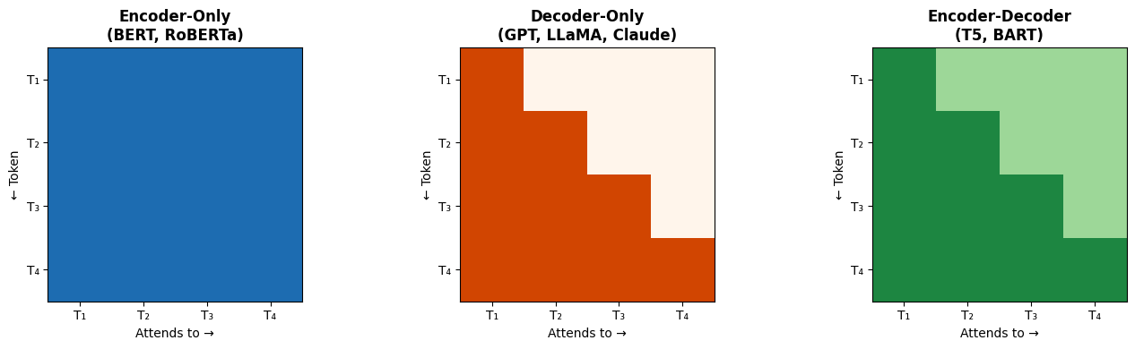
Architecture Comparison
Table 1:Transformer Model Variants Compared
| Encoder-Only | Decoder-Only | Encoder-Decoder | |
|---|---|---|---|
| Architecture | Encoder stack only | Decoder stack only | Both stacks + cross-attention |
| Attention | Bidirectional (full) | Causal (left-to-right) | Bidirectional encoder, causal decoder |
| Pretraining | Masked Language Modeling | Next-token prediction | Span corruption or denoising |
| Strengths | Understanding, classification, extraction | Generation, few-shot, in-context learning | Sequence-to-sequence transformation |
| Limitations | Cannot generate text | Misses right context at each position | More parameters, higher complexity |
| Canonical Models | BERT, RoBERTa, DeBERTa | GPT-3/4, LLaMA, Claude, Gemini | T5, BART, mBART |
| Use When... | You need to classify, extract, or compare | You need to generate or converse | Input → different output (translate, summarize) |

Figure 6:A practical decision tree for choosing the right transformer architecture based on your NLP task.
The Trend: Decoder-Only Dominance
If you look at the most capable models today — GPT-4, Claude, LLaMA, Gemini — they are all decoder-only. This doesn’t mean encoder-only and encoder-decoder models are obsolete. Rather, the landscape has evolved:
Encoder-only models (RoBERTa, DeBERTa) are still the go-to for efficient, task-specific deployments. If you need a fast sentiment classifier or NER system, fine-tuning a relatively small encoder-only model is far more cost-effective than running every request through a massive LLM.
Encoder-decoder models (T5, BART) remain competitive for structured transformation tasks like translation and summarization, especially in research settings.
Decoder-only models dominate when you want a general-purpose model that handles many tasks through prompting, or when you need open-ended generation.
The key takeaway is that architecture choice is a design decision driven by your task, your constraints, and your deployment context. Understanding all three variants lets you make that decision wisely.
Wrap-Up
Key Takeaways
What’s Next
In Part 02, we’ll get hands-on with the Hugging Face ecosystem — the toolkit that makes all three of these model families accessible through a unified Python API. You’ll learn to load pretrained models and tokenizers from the Hugging Face Hub, use high-level pipelines for rapid prototyping, and work with the Datasets library for loading and processing data. The conceptual understanding of model variants you’ve built today will directly inform which models you reach for and why.